Reference genome files

Downloading & exploring FASTA and GTF files in the shell,
including with grep, cut, sort, and uniq

Author

Jelmer Poelstra

Published

August 11, 2023

Overview & setting up

In this session, we’ll talk about the two main types of reference genome files that you need in a reference-based RNAseq analysis (and other reference-genome based genomics analysis like variant calling): FASTA and GTF/GFF.

FASTA files: Simple sequence files, where each entry contains just a header and a DNA or protein sequence. Your reference genome assembly will be in this format.
GTF (& GFF) files: These contain annotations in a tabular format, e.g. the start & stop position of each gene.

We will download these files from the internet using wget, and will also see a few new shell commands that can be used to summarize tabular data like that in GTF files: cut, sort, and uniq (in combination with grep).

Start VS Code and open your folder

As always, we’ll be working in VS Code — if you don’t already have a session open, see below how to do so.

Make sure to open your /fs/ess/PAS0471/<user>/rnaseq_intro dir, either by using the Open Folder menu item, or by clicking on this dir when it appears in the Welcome tab.

Starting VS Code at OSC - with a Terminal (Click to expand)

Log in to OSC’s OnDemand portal at https://ondemand.osc.edu.
In the blue top bar, select Interactive Apps and then near the bottom of the dropdown menu, click Code Server.
In the form that appears on a new page:
- Select an appropriate OSC project (here: PAS0471)
- For this session, select /fs/ess/PAS0471 as the starting directory
- Make sure that Number of hours is at least 2
- Click Launch.
On the next page, once the top bar of the box has turned green and says Runnning, click Connect to VS Code.

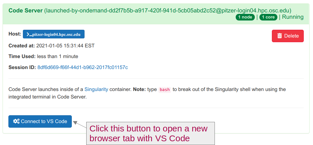
Open a Terminal by clicking => Terminal => New Terminal. (Or use one of the keyboard shortcuts: Ctrl+` (backtick) or Ctrl+Shift+C.)
In the Welcome tab under Recent, you should see your /fs/ess/PAS0471/<user>/rnaseq_intro dir listed: click on that to open it. Alternatively, use => File => Open Folder to open that dir in VS Code.

Don’t have your own dir with the data? (Click to expand)

If you missed the last session, or deleted your rnaseq_intro dir entirely, run these commands to get a (fresh) copy of all files:

mkdir -p /fs/ess/PAS0471/$USER/rnaseq_intro
cp -r /fs/ess/PAS0471/demo/202307_rnaseq /fs/ess/PAS0471/$USER/rnaseq_intro

And if you do have an rnaseq_intro dir, but you want to start over because you moved or removed some of the files while practicing, then delete the dir before your run the commands above:

rm -r /fs/ess/PAS0471/$USER/rnaseq_intro

You should have at least the following files in this dir:

/fs/ess/PAS0471/demo/202307_rnaseq
├── data
│   └── fastq
│       ├── ASPC1_A178V_R1.fastq.gz
│       ├── ASPC1_A178V_R2.fastq.gz
│       ├── ASPC1_G31V_R1.fastq.gz
│       ├── ASPC1_G31V_R2.fastq.gz
│       ├── Miapaca2_A178V_R1.fastq.gz
│       ├── Miapaca2_A178V_R2.fastq.gz
│       ├── Miapaca2_G31V_R1.fastq.gz
│       └── Miapaca2_G31V_R2.fastq.gz
├── metadata
│   └── meta.tsv
└── README.md

1 Downloading reference genome files

1.1 Finding genome files at NCBI

To analyze our RNAseq data, we’ll need two files related to our reference genome. This is the genome that we will align our reads to, and whose gene annotations will form the basis of the gene counts we’ll eventually get.

Specifically, we’ll need the nucleotide FASTA file with the genome assembly itself, and a GTF file, which is a tabular file with the genomic coordinates and other information for genes and other so-called genomic “features”.

We can download these files from NCBI. For human, many genome assemblies are available on NCBI, but the current reference genome is “GRCh38.p14” (see this overview). There are several ways to download genomes from the NCBI — here, we will keep it simple and directly download just the two files that we need from the NCBI FTP site for this genome.

Getting to the FTP site

You can get to this FTP site by clicking on the link for “GRCh38.p14” on the overview page, which will bring you here, then clicking on “View the legacy Assembly page”, which will bring you here, and then clicking on “FTP directory for RefSeq assembly” on the right-hand side of the page.

On the FTP site, right-click on GCF_000001405.40_GRCh38.p14_genomic.fna.gz and then click “Copy link address” (the URL to this file is also shown in the command box below).

1.2 Downloading files to OSC with `wget`

To download a file to OSC, you can’t just open a web browser and download it there directly. You could download it to your own computer and then transfer it to OSC. A more direct approach is to use a download command in your OSC shell. wget is one command that allows you to download files from the web¹.

To download a file to your working directory, you just need to tell wget about the URL (web address) to that file — type “wget”, press Space, and paste the address you copied:

wget https://ftp.ncbi.nlm.nih.gov/genomes/all/GCF/000/001/405/GCF_000001405.40_GRCh38.p14/GCF_000001405.40_GRCh38.p14_genomic.fna.gz

--2023-08-08 13:46:35--  https://ftp.ncbi.nlm.nih.gov/genomes/all/GCF/000/001/405/GCF_000001405.40_GRCh38.p14/GCF_000001405.40_GRCh38.p14_genomic.fna.gz
Resolving ftp.ncbi.nlm.nih.gov (ftp.ncbi.nlm.nih.gov)... 130.14.250.11, 130.14.250.10, 2607:f220:41e:250::12, ...
Connecting to ftp.ncbi.nlm.nih.gov (ftp.ncbi.nlm.nih.gov)|130.14.250.11|:443... connected.
HTTP request sent, awaiting response... 200 OK
Length: 972898531 (928M) [application/x-gzip]
Saving to: ‘GCF_000001405.40_GRCh38.p14_genomic.fna.gz’
65% [============================================================================================>                                                   ] 633,806,848 97.7MB/s

The wget command is quite chatty, as you can see above, and its output to the screen includes a progress bar for the download.

Next, let’s download one of the annotation files. On the NCBI genome assembly FTP page, both a GFF and a GTF file are available. These are two very similar formats that contain the same data. For our specific analysis workflow, the GTF format is preferred, so we will download the GTF file — right-click on GCF_000001405.40_GRCh38.p14_genomic.gtf.gz and copy the link address.

wget https://ftp.ncbi.nlm.nih.gov/genomes/all/GCF/000/001/405/GCF_000001405.40_GRCh38.p14/GCF_000001405.40_GRCh38.p14_genomic.gtf.gz
# (Command output not shown)

Next, let’s see if the files are indeed in our current working dir:

ls -lh

# (Output should include:)
-rw-r--r-- 1 jelmer PAS0471 928M Mar 21 10:15 GCF_000001405.40_GRCh38.p14_genomic.fna.gz
-rw-r--r-- 1 jelmer PAS0471  49M Mar 21 10:15 GCF_000001405.40_GRCh38.p14_genomic.gtf.gz

1.3 Uncompressing and renaming the genome files

Both the FASTA and the GTF file are gzip-compressed. While it’s preferable to keep FASTQ files compressed (as mentioned above), it’s often more convenient to store your reference genome files as uncompressed files².

We can uncompress/unzip these files with the gunzip (“g-unzip”) command as follows (and notice the subsequent increase in file size in the ls output):

# Will take several seconds, esp. for the first file, and not print output to screen
gunzip GCF_000001405.40_GRCh38.p14_genomic.fna.gz
gunzip GCF_000001405.40_GRCh38.p14_genomic.gtf.gz

ls -lh

# (Output should include:)
-rw-r--r-- 1 jelmer PAS0471 3.2G Mar 21 10:15 GCF_000001405.40_GRCh38.p14_genomic.fna
-rw-r--r-- 1 jelmer PAS0471 1.6G Mar 21 10:15 GCF_000001405.40_GRCh38.p14_genomic.gtf

We’ll also want to move these files to a dedicated directory. Also, it will be convenient for our purposes to shorten their file names while retaining the necessary identifying information (the “GCF_” RefSeq number).

After creating a directory, we can move and rename the files at once as follows:

# We'll use a dir 'data/ref' for reference genome files
mkdir -p data/ref

mv -v GCF_000001405.40_GRCh38.p14_genomic.fna data/ref/GCF_000001405.40.fna
mv -v GCF_000001405.40_GRCh38.p14_genomic.gtf data/ref/GCF_000001405.40.gtf

‘GCF_000001405.40_GRCh38.p14_genomic.fna’ -> ‘data/ref/GCF_000001405.40.fna’
‘GCF_000001405.40_GRCh38.p14_genomic.gtf’ -> ‘data/ref/GCF_000001405.40.gtf’

2 FASTA

Our reference genome assembly is stored in the FASTA format, so we’ll learn more about this format and take a look at our own file.

2.1 The FASTA format

The FASTA format is in essence simpler than FASTQ, but it is also less standardized and more generic.

The following example FASTA file contains two entries:

>unique_sequence_ID Optional description (free form!)
ATTCATTAAAGCAGTTTATTGGCTTAATGTACATCAGTGAAATCATAAATGCTAAAAA
>unique_sequence_ID2
ATTCATTAAAGCAGTTTATTGGCTTAATGTACATCAGTGAAATCATAAATGCTAAATG

Like FASTQ files, each entry contains a header and the sequence itself, but:

Header lines start with a > and are otherwise basically “free form”, but they usually provide some sort of identifier (and sometimes some metadata) for the sequence in the entry.
There are no quality scores, and there is no + line.
The sequences can be DNA, RNA, or amino acids.
A FASTA entry can represent a number of different types of sequencs, such as a read, a contig/scaffold, a chromosome, or a gene, as well as an aligned sequence with gaps in it.
Because the individual sequences in a FASTA file can be very long, sequences are often not on a single line, but may be spread across multiple/many lines with some fixed width, say 50 or 80 characters. (As such, line counts are not that informative!)

Generic FASTA file extensions are .fasta and .fa, but also used are extensions that explicitly indicate whether the sequences are nucleotides (.fna, like our downloaded genome assembly file) or amino acids (.faa).

2.2 Exploring our FASTA file

Let’s take a look at the first lines of our reference genome FASTA:

head data/ref/GCF_000001405.40.fna

>NC_000001.11 Homo sapiens chromosome 1, GRCh38.p14 Primary Assembly
NNNNNNNNNNNNNNNNNNNNNNNNNNNNNNNNNNNNNNNNNNNNNNNNNNNNNNNNNNNNNNNNNNNNNNNNNNNNNNNN
NNNNNNNNNNNNNNNNNNNNNNNNNNNNNNNNNNNNNNNNNNNNNNNNNNNNNNNNNNNNNNNNNNNNNNNNNNNNNNNN
NNNNNNNNNNNNNNNNNNNNNNNNNNNNNNNNNNNNNNNNNNNNNNNNNNNNNNNNNNNNNNNNNNNNNNNNNNNNNNNN
NNNNNNNNNNNNNNNNNNNNNNNNNNNNNNNNNNNNNNNNNNNNNNNNNNNNNNNNNNNNNNNNNNNNNNNNNNNNNNNN
NNNNNNNNNNNNNNNNNNNNNNNNNNNNNNNNNNNNNNNNNNNNNNNNNNNNNNNNNNNNNNNNNNNNNNNNNNNNNNNN
NNNNNNNNNNNNNNNNNNNNNNNNNNNNNNNNNNNNNNNNNNNNNNNNNNNNNNNNNNNNNNNNNNNNNNNNNNNNNNNN
NNNNNNNNNNNNNNNNNNNNNNNNNNNNNNNNNNNNNNNNNNNNNNNNNNNNNNNNNNNNNNNNNNNNNNNNNNNNNNNN
NNNNNNNNNNNNNNNNNNNNNNNNNNNNNNNNNNNNNNNNNNNNNNNNNNNNNNNNNNNNNNNNNNNNNNNNNNNNNNNN
NNNNNNNNNNNNNNNNNNNNNNNNNNNNNNNNNNNNNNNNNNNNNNNNNNNNNNNNNNNNNNNNNNNNNNNNNNNNNNNN

Well … apparently not all bases have been determined: as you probably know, an N represents an unknown base. We can also see that the sequence for each entry is spread across multiple lines, with a line width of 80 characters:

# 'head -n 2 | tail -n 1' prints the second line; 'wc -c' counts characters
head -n 2 data/ref/GCF_000001405.40.fna | tail -n 1 | wc -c

81              # 81 - 1 = 80 characters

Let’s take a more extensive look at the file with less:

less data/ref/GCF_000001405.40.fna
# (Remember: press 'q' to quit less)

We can also look at all or some of the entry headers by greping for > (which is only allowed in the header) — in this file, we can see that the entries represent the scaffolds:

grep ">" data/ref/GCF_000001405.40.fna | head

>NC_000001.11 Homo sapiens chromosome 1, GRCh38.p14 Primary Assembly
>NT_187361.1 Homo sapiens chromosome 1 unlocalized genomic scaffold, GRCh38.p14 Primary Assembly HSCHR1_CTG1_UNLOCALIZED
>NT_187362.1 Homo sapiens chromosome 1 unlocalized genomic scaffold, GRCh38.p14 Primary Assembly HSCHR1_CTG2_UNLOCALIZED
>NT_187363.1 Homo sapiens chromosome 1 unlocalized genomic scaffold, GRCh38.p14 Primary Assembly HSCHR1_CTG3_UNLOCALIZED
>NT_187364.1 Homo sapiens chromosome 1 unlocalized genomic scaffold, GRCh38.p14 Primary Assembly HSCHR1_CTG4_UNLOCALIZED
>NT_187365.1 Homo sapiens chromosome 1 unlocalized genomic scaffold, GRCh38.p14 Primary Assembly HSCHR1_CTG5_UNLOCALIZED
>NT_187366.1 Homo sapiens chromosome 1 unlocalized genomic scaffold, GRCh38.p14 Primary Assembly HSCHR1_CTG6_UNLOCALIZED
>NT_187367.1 Homo sapiens chromosome 1 unlocalized genomic scaffold, GRCh38.p14 Primary Assembly HSCHR1_CTG7_UNLOCALIZED
>NT_187368.1 Homo sapiens chromosome 1 unlocalized genomic scaffold, GRCh38.p14 Primary Assembly HSCHR1_CTG8_UNLOCALIZED
>NT_187369.1 Homo sapiens chromosome 1 unlocalized genomic scaffold, GRCh38.p14 Primary Assembly HSCHR1_CTG9_UNLOCALIZED

Finally, let’s count the number of scaffolds simply by counting the number of lines with a >:

# (This will take several seconds)
grep -c ">" data/ref/GCF_000001405.40.fna

Does this match with what the NCBI website told us?

3 Annotation files (GTF/GFF)

Our reference genome annotation is stored in the GTF format, so we’ll learn about this format, too, and take a look at our own file.

3.1 The GTF format

The GTF format and the very similar GFF format³ are tabular files, with one row for each individual “genomic feature” (gene, exon, intron, etc.) that has been annotated in the genome, and with columns that contain information like the genomic coordinates of the features.

See the small sample below, with an added header line (not normally present) with column names for clarity:

seqname     source  feature start   end     score  strand  frame    attributes
NC_000001   RefSeq  gene    11874   14409   .       +       .       gene_id "DDX11L1"; transcript_id ""; db_xref "GeneID:100287102"; db_xref "HGNC:HGNC:37102"; description "DEAD/H-box helicase 11 like 1 (pseudogene)"; gbkey "Gene"; gene "DDX11L1"; gene_biotype "transcribed_pseudogene"; pseudo "true"; 
NC_000001   RefSeq  exon    11874   12227   .       +       .       gene_id "DDX11L1"; transcript_id "NR_046018.2"; db_xref "GeneID:100287102"; gene "DDX11L1"; product "DEAD/H-box helicase 11 like 1 (pseudogene)"; pseudo "true";

Here are some more details on what’s in each column, with the more important/interesting columns in bold:

seqname — Name of the chromosome, scaffold, or contig
source — Name of the program that generated this feature, or the data source (e.g. database)
feature — Name of the feature type, e.g. “gene”, “exon”, “intron”, “CDS”
start — Start position of the feature (sequence numbering starts at 1; start position is included)
end — End position of the feature (end position is also included)
score — A confidence score for the feature, often absent (in which case it is .)
strand — Whether the feature is on the + (forward) or - (reverse) strand
frame — 0, 1 or 2 (or . for no frame). 0 means the 1st base of the feature is the 1st base of a codon, etc.
attribute — A semicolon-separated list of tag-value pairs with additional information about each feature.

As we’ll see below, GTF files also have a header section, whose lines start with a # and contain some metadata for the file.

Annotation and assembly versions

Because GTF/GFF files contain genomic coordinates, it is essential that the FASTA and GTF/GFF you are working with correspond to the same assembly. For example, if you want to use an updated assembly FASTA for your focal genome, you’re going to need an updated annotation file as well. (On the other hand, it is possible to update just the annotation for the same assembly.)

3.2 Exploring our GTF file

Let’s take a look at the first lines of the file with head, which shows us that there are five header lines, followed by the tabular part of the file:

head data/ref/GCF_000001405.40.gtf

#gtf-version 2.2
#!genome-build GRCh38.p14
#!genome-build-accession NCBI_Assembly:GCF_000001405.40
#!annotation-date 03/15/2023
#!annotation-source NCBI RefSeq GCF_000001405.40-RS_2023_03
NC_000001.11    BestRefSeq      gene    11874   14409   .       +       .       gene_id "DDX11L1"; transcript_id ""; db_xref "GeneID:100287102"; db_xref "HGNC:HGNC:37102"; description "DEAD/H-box helicase 11 like 1 (pseudogene)"; gbkey "Gene"; gene "DDX11L1"; gene_biotype "transcribed_pseudogene"; pseudo "true"; 
NC_000001.11    BestRefSeq      transcript      11874   14409   .       +       .       gene_id "DDX11L1"; transcript_id "NR_046018.2"; db_xref "GeneID:100287102"; gbkey "misc_RNA"; gene "DDX11L1"; product "DEAD/H-box helicase 11 like 1 (pseudogene)"; pseudo "true"; transcript_biotype "transcript"; 
NC_000001.11    BestRefSeq      exon    11874   12227   .       +       .       gene_id "DDX11L1"; transcript_id "NR_046018.2"; db_xref "GeneID:100287102"; gene "DDX11L1"; product "DEAD/H-box helicase 11 like 1 (pseudogene)"; pseudo "true"; transcript_biotype "transcript"; exon_number "1"; 
NC_000001.11    BestRefSeq      exon    12613   12721   .       +       .       gene_id "DDX11L1"; transcript_id "NR_046018.2"; db_xref "GeneID:100287102"; gene "DDX11L1"; product "DEAD/H-box helicase 11 like 1 (pseudogene)"; pseudo "true"; transcript_biotype "transcript"; exon_number "2"; 
NC_000001.11    BestRefSeq      exon    13221   14409   .       +       .       gene_id "DDX11L1"; transcript_id "NR_046018.2"; db_xref "GeneID:100287102"; gene "DDX11L1"; product "DEAD/H-box helicase 11 like 1 (pseudogene)"; pseudo "true"; transcript_biotype "transcript"; exon_number "3";

The final column (“attributes”) contains lots of data, so the line width will almost certainly exceed your screen width, and the output you see in your shell will be line-wrapped. It’s easier to see what’s going on on this website (where we get one line for each line of the file, and can scroll sideways), or with less -S:

less -S data/ref/GCF_000001405.40.gtf

One nice trick for if we only want to only see the tabular lines (for some files, the header can be quite long), or if we want to summarize the data in the tabular lines, is to omit the header lines using grep -v. The -v option will invert grep’s behavior and only print non-matching lines — since only the header lines contain a #, we can use that as the pattern to search for:

grep -v "#" data/ref/GCF_000001405.40.gtf | head -n 3

NC_000001.11    BestRefSeq      gene    11874   14409   .       +       .       gene_id "DDX11L1"; transcript_id ""; db_xref "GeneID:100287102"; db_xref "HGNC:HGNC:37102"; description "DEAD/H-box helicase 11 like 1 (pseudogene)"; gbkey "Gene"; gene "DDX11L1"; gene_biotype "transcribed_pseudogene"; pseudo "true"; 
NC_000001.11    BestRefSeq      transcript      11874   14409   .       +       .       gene_id "DDX11L1"; transcript_id "NR_046018.2"; db_xref "GeneID:100287102"; gbkey "misc_RNA"; gene "DDX11L1"; product "DEAD/H-box helicase 11 like 1 (pseudogene)"; pseudo "true"; transcript_biotype "transcript"; 
NC_000001.11    BestRefSeq      exon    11874   12227   .       +       .       gene_id "DDX11L1"; transcript_id "NR_046018.2"; db_xref "GeneID:100287102"; gene "DDX11L1"; product "DEAD/H-box helicase 11 like 1 (pseudogene)"; pseudo "true"; transcript_biotype "transcript"; exon_number "1";

This will also allow us to count the number of annotated features in the genome (4,684,284):

grep -cv "#" data/ref/GCF_000001405.40.gtf

Let’s see if we can find a gene of interest, “RASD1” in this annotation:

grep "RASD1" data/ref/GCF_000001405.40.gtf

NC_000017.11    BestRefSeq      gene    17494437        17496395        .       -       .       gene_id "RASD1"; transcript_id ""; db_xref "GeneID:51655"; db_xref "HGNC:HGNC:15828"; db_xref "MIM:605550"; description "ras related dexamethasone induced 1"; gbkey "Gene"; gene "RASD1"; gene_biotype "protein_coding"; gene_synonym "AGS1"; gene_synonym "DEXRAS1"; gene_synonym "MGC:26290"; 
NC_000017.11    BestRefSeq      transcript      17494437        17496395        .       -       .       gene_id "RASD1"; transcript_id "NM_001199989.2"; db_xref "GeneID:51655"; gbkey "mRNA"; gene "RASD1"; product "ras related dexamethasone induced 1, transcript variant 2"; transcript_biotype "mRNA"; 
NC_000017.11    BestRefSeq      exon    17495896        17496395        .       -       .       gene_id "RASD1"; transcript_id "NM_001199989.2"; db_xref "GeneID:51655"; gene "RASD1"; product "ras related dexamethasone induced 1, transcript variant 2"; transcript_biotype "mRNA"; exon_number "1"; 
NC_000017.11    BestRefSeq      exon    17494437        17495610        .       -       .       gene_id "RASD1"; transcript_id "NM_001199989.2"; db_xref "GeneID:51655"; gene "RASD1"; product "ras related dexamethasone induced 1, transcript variant 2"; transcript_biotype "mRNA"; exon_number "2"; 
NC_000017.11    BestRefSeq      CDS     17495896        17496181        .       -       0       gene_id "RASD1"; transcript_id "NM_001199989.2"; db_xref "CCDS:CCDS58519.1"; db_xref "GeneID:51655"; gbkey "CDS"; gene "RASD1"; note "isoform 2 is encoded by transcript variant 2"; product "dexamethasone-induced Ras-related protein 1 isoform 2"; protein_id "NP_001186918.1"; exon_number "1"; 
NC_000017.11    BestRefSeq      CDS     17495531        17495610        .       -       2       gene_id "RASD1"; transcript_id "NM_001199989.2"; db_xref "CCDS:CCDS58519.1"; db_xref "GeneID:51655"; gbkey "CDS"; gene "RASD1"; note "isoform 2 is encoded by transcript variant 2"; product "dexamethasone-induced Ras-related protein 1 isoform 2"; protein_id "NP_001186918.1"; exon_number "2"; 
NC_000017.11    BestRefSeq      start_codon     17496179        17496181        .       -       0       gene_id "RASD1"; transcript_id "NM_001199989.2"; db_xref "CCDS:CCDS58519.1"; db_xref "GeneID:51655"; gbkey "CDS"; gene "RASD1"; note "isoform 2 is encoded by transcript variant 2"; product "dexamethasone-induced Ras-related protein 1 isoform 2"; protein_id "NP_001186918.1"; exon_number "1"; 
NC_000017.11    BestRefSeq      stop_codon      17495528        17495530        .       -       0       gene_id "RASD1"; transcript_id "NM_001199989.2"; db_xref "CCDS:CCDS58519.1"; db_xref "GeneID:51655"; gbkey "CDS"; gene "RASD1"; note "isoform 2 is encoded by transcript variant 2"; product "dexamethasone-induced Ras-related protein 1 isoform 2"; protein_id "NP_001186918.1"; exon_number "2"; 
NC_000017.11    BestRefSeq      transcript      17494437        17496395        .       -       .       gene_id "RASD1"; transcript_id "NM_016084.5"; db_xref "Ensembl:ENST00000225688.4"; db_xref "GeneID:51655"; gbkey "mRNA"; gene "RASD1"; product "ras related dexamethasone induced 1, transcript variant 1"; tag "MANE Select"; transcript_biotype "mRNA"; 
NC_000017.11    BestRefSeq      exon    17495896        17496395        .       -       .       gene_id "RASD1"; transcript_id "NM_016084.5"; db_xref "Ensembl:ENST00000225688.4"; db_xref "GeneID:51655"; gene "RASD1"; product "ras related dexamethasone induced 1, transcript variant 1"; tag "MANE Select"; transcript_biotype "mRNA"; exon_number "1"; 
NC_000017.11    BestRefSeq      exon    17494437        17495684        .       -       .       gene_id "RASD1"; transcript_id "NM_016084.5"; db_xref "Ensembl:ENST00000225688.4"; db_xref "GeneID:51655"; gene "RASD1"; product "ras related dexamethasone induced 1, transcript variant 1"; tag "MANE Select"; transcript_biotype "mRNA"; exon_number "2"; 
NC_000017.11    BestRefSeq      CDS     17495896        17496181        .       -       0       gene_id "RASD1"; transcript_id "NM_016084.5"; db_xref "CCDS:CCDS11185.1"; db_xref "Ensembl:ENSP00000225688.3"; db_xref "GeneID:51655"; gbkey "CDS"; gene "RASD1"; note "isoform 1 proprotein is encoded by transcript variant 1"; product "dexamethasone-induced Ras-related protein 1 isoform 1 proprotein"; protein_id "NP_057168.1"; tag "MANE Select"; exon_number "1"; 
NC_000017.11    BestRefSeq      CDS     17495128        17495684        .       -       2       gene_id "RASD1"; transcript_id "NM_016084.5"; db_xref "CCDS:CCDS11185.1"; db_xref "Ensembl:ENSP00000225688.3"; db_xref "GeneID:51655"; gbkey "CDS"; gene "RASD1"; note "isoform 1 proprotein is encoded by transcript variant 1"; product "dexamethasone-induced Ras-related protein 1 isoform 1 proprotein"; protein_id "NP_057168.1"; tag "MANE Select"; exon_number "2"; 
NC_000017.11    BestRefSeq      start_codon     17496179        17496181        .       -       0       gene_id "RASD1"; transcript_id "NM_016084.5"; db_xref "CCDS:CCDS11185.1"; db_xref "Ensembl:ENSP00000225688.3"; db_xref "GeneID:51655"; gbkey "CDS"; gene "RASD1"; note "isoform 1 proprotein is encoded by transcript variant 1"; product "dexamethasone-induced Ras-related protein 1 isoform 1 proprotein"; protein_id "NP_057168.1"; tag "MANE Select"; exon_number "1"; 
NC_000017.11    BestRefSeq      stop_codon      17495125        17495127        .       -       0       gene_id "RASD1"; transcript_id "NM_016084.5"; db_xref "CCDS:CCDS11185.1"; db_xref "Ensembl:ENSP00000225688.3"; db_xref "GeneID:51655"; gbkey "CDS"; gene "RASD1"; note "isoform 1 proprotein is encoded by transcript variant 1"; product "dexamethasone-induced Ras-related protein 1 isoform 1 proprotein"; protein_id "NP_057168.1"; tag "MANE Select"; exon_number "2";

That worked! We are getting quite a few lines, but these are all features for one single gene (there is only a single gene feature, in the first line).

4 Summarizing tabular data with shell tools

4.1 Introduction to `cut`, `uniq`, and `sort`

Using more grep as well as a few new shell commands, we can quickly get some useful information about the GTF file. Let’s learn about cut, sort, and uniq using our metadata file, which has the following content:

# (Column -t is useful for displaying tabular files with columns aligned)
column -t metadata/meta.tsv

sample_id       cell_line  variant
ASPC1_A178V     ASPC1      A178V
ASPC1_A178V     ASPC1      A178V
ASPC1_G31V      ASPC1      G31V
ASPC1_G31V      ASPC1      G31V
Miapaca2_A178V  Miapaca2   A178V
Miapaca2_A178V  Miapaca2   A178V
Miapaca2_G31V   Miapaca2   G31V
Miapaca2_G31V   Miapaca2   G31V

First, the cut command can extract columns from tabular files, and you can use its -f option to specify the column(s) you want to extract — for example, -f 3 extracts column 3, while -f 3,5 would extract columns 3 and 5:

cut -f 3 metadata/meta.tsv

variant
A178V
A178V
G31V
G31V
A178V
A178V
G31V
G31V

Second, the sort command will sort its input:

cut -f 3 metadata/meta.tsv | sort

A178V
A178V
A178V
A178V
G31V
G31V
G31V
G31V
variant

Other sort functionality

While in the example below, we’re sorting a single column, sort can also sort multi-column files on one or more columns, while keeping the rows intact. Additionally, it can sort numerically, in reverse, and much more.

Hmmm… maybe it isn’t appropriate to include the header line (variant in the output above). A nice little trick to exclude the first line of a file is tail -n +2:

tail -n +2 metadata/meta.tsv | cut -f 3 | sort

A178V
A178V
A178V
A178V
G31V
G31V
G31V
G31V

Third, the uniq command will remove consecutive duplicate lines — for that reason, its input needs to be sorted if we want to remove all duplicates:

tail -n +2 metadata/meta.tsv | cut -f 3 | sort | uniq

A178V
G31V

For large input files, it’s most often useful to either:

Simply get the number of unique values that occur in a column by piping into wc -l:

tail -n +2 metadata/meta.tsv | cut -f 3 | sort | uniq | wc -l

Get a “count table” showing how many times each value in a column occurs using uniq’s -c option:

tail -n +2 metadata/meta.tsv | cut -f 3 | sort | uniq -c

      4 A178V
      4 G31V

4.2 Getting GTF summary stats with `cut`, `uniq`, and `grep`

How many snRNAs are in the annotation?

# Because the 'gene_biotype' attribute only occurs in 'gene' entries,
# we can simply count the number of lines found by grep:
grep -c 'gene_biotype "snRNA"' data/ref/GCF_000001405.40.gtf

How many “RASD” genes are in the annotation?

# After getting all RASD entries (for different feature types), we can select
# only 'gene' entries by cutting column 3 (feature types) and grep for 'gene':
grep 'gene_id "RASD' data/ref/GCF_000001405.40.gtf | cut -f 3 | grep -c "gene"

Which feature types are present and what are their counts?

# Column 3 contains the feature types
grep -v "^#" data/ref/GCF_000001405.40.gtf | cut -f 3 | sort | uniq -c

1835339 CDS
2291763 exon
  67127 gene
 145185 start_codon
 144753 stop_codon
 200121 transcript

Your turn: more GTF exploration

How many features are derived from each of the annotation sources (column 2)?

Hint

The code to do this is nearly identical to the last example above, you just have to cut a different column.

Solution

grep -v "#" $gtf | cut -f 2 | sort | uniq -c

2141089 BestRefSeq
  11308 BestRefSeq%2CGnomon
   2955 cmsearch
  21999 Curated Genomic
2504737 Gnomon
    150 RefSeq
   2050 tRNAscan-SE

Above, we got counts of features by type (gene, exon, etc., in column 3). Now, get separate counts of each feature type on each strand.