Lab: Running the nf-core rnaseq pipeline

Author

Jelmer Poelstra

Published

January 27, 2025

1 Introduction

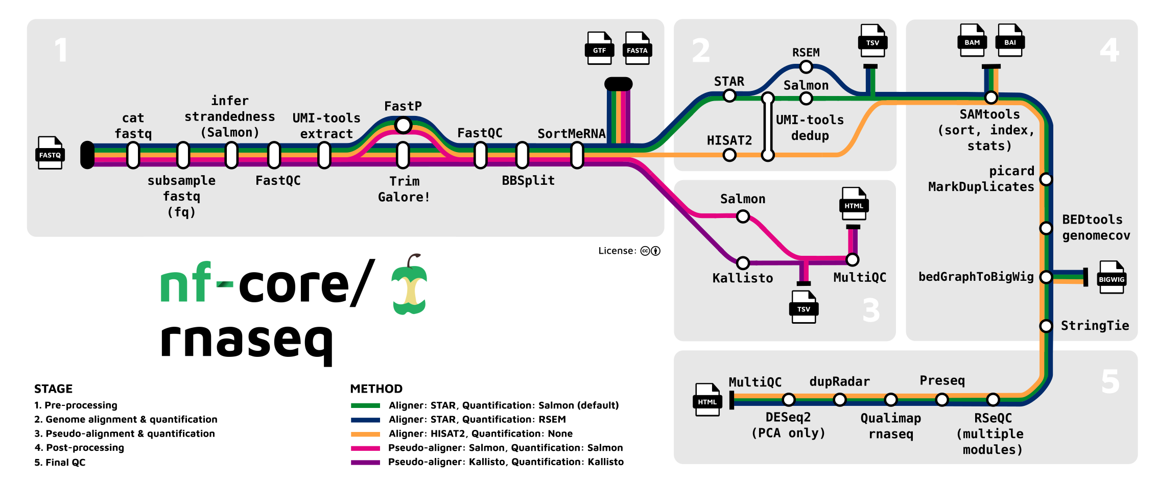
In this tutorial, we will run the nf-core rnaseq pipeline. Using raw RNA-seq reads in FASTQ files and reference genomes files as inputs, this pipeline will generate a gene count table as its most important output. That gene count table can then be analyzed to examine, for example, differential expression, which is the topic of the self-study lab.

An overview of the steps in the nf-core rnaseq pipeline.

We will work with the data set from the paper “Two avian Plasmodium species trigger different transcriptional responses on their vector Culex pipiens”, published last year in Molecular Ecology (link):

This paper uses RNA-seq data to study gene expression in Culex pipiens mosquitoes infected with malaria-causing Plasmodium protozoans — specifically, it compares mosquito according to:

Infection status: Plasmodium cathemerium vs. P. relictum vs. control
Time after infection: 24 h vs. 10 days vs. 21 days

2 Getting started with VS Code

We will use the VS Code text editor to write a script to run the nf-core rnaseq pipeline. To emphasize the additional functionality relative to basic text editors like Notepad and TextEdit, editors like VS Code are also referred to as “IDEs”: Integrated Development Environments. The RStudio program is another good example of an IDE. Just like RStudio is an IDE for R, VS Code will be our IDE for shell code today.

2.1 Starting VS Code at OSC

Log in to OSC’s OnDemand portal at https://ondemand.osc.edu.
In the blue top bar, select Interactive Apps and near the bottom, click Code Server.
VS Code runs on a compute node so we have to fill out a form to make a reservation for one:
- The OSC “Project” that we want to bill for the compute node usage: PAS2658.
- The “Number of hours” we want to make a reservation for: 2.
- The “Working Directory” for the program: your personal folder in /fs/scratch/PAS2658 (e.g. /fs/scratch/PAS2658/jelmer).
- The “Codeserver Version”: 4.8 (most recent).
- Click Launch.
First, your job will be “Queued” — that is, waiting for the job scheduler to allocate compute node resources to it.
Your job is typically granted resources within a few seconds (the card will then say “Starting”), and should be ready for usage (“Running”) in another couple of seconds. Once the job is running click on the blue Connect to VS Code button to open VS Code — it will open in a new browser tab.
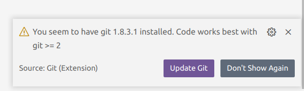
When VS Code opens, you may get these two pop-ups (and possibly some others) — click “Yes” (and check the box) and “Don’t Show Again”, respectively:

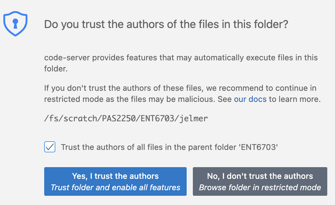
You’ll also get a Welcome/Get Started page — you don’t have to go through steps that may be suggested there.

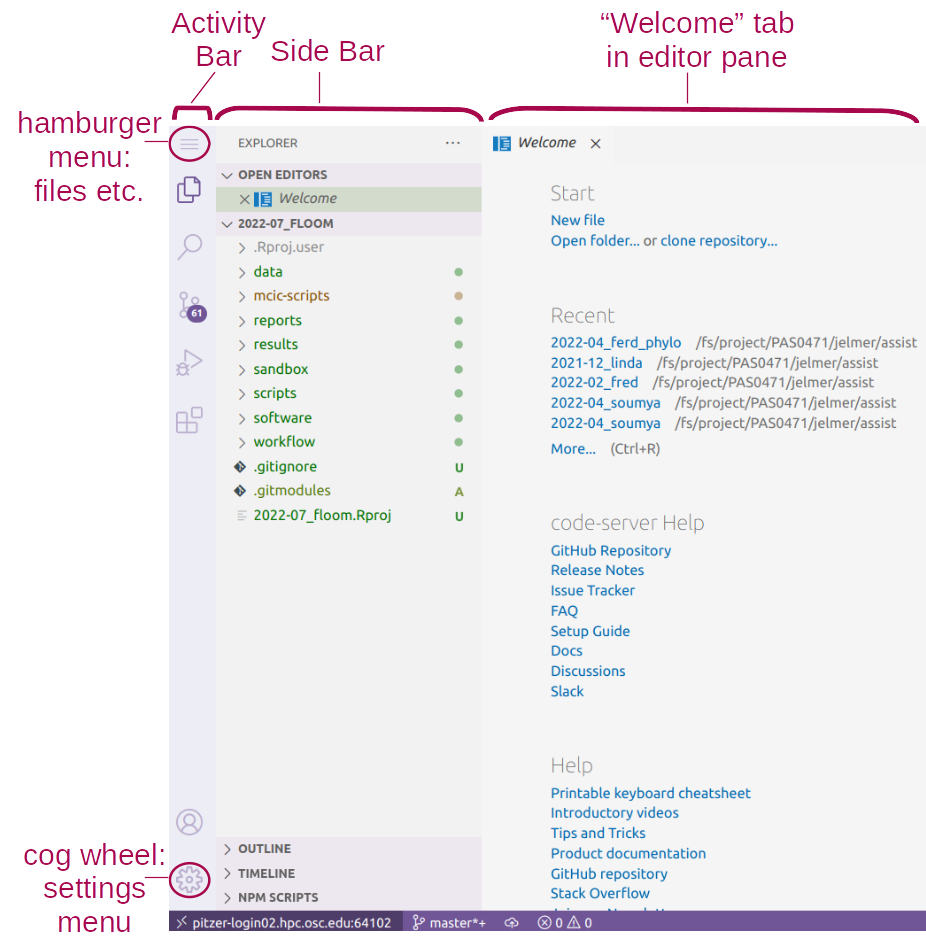
2.2 The VS Code User Interface

Click to see an annotated screenshot

Side bars

The narrow side bar on the far left has:

A (“hamburger menu”), which has menu items like File that you often find in a top bar.
A (cog wheel icon) in the bottom, through which you can mainly access settings.
Icons to toggle between options for what to show in the wide side bar, e.g. a File Explorer (the default option).

Terminal

Open a terminal with a Unix shell: click => Terminal => New Terminal. In the terminal, create a dir for this lab, e.g.:

# You should be in your personal dir in /fs/scratch/PAS2658
pwd

/fs/scratch/PAS2658/jelmer

mkdir -p Lab9 
cd Lab9
mkdir scripts run software

Editor pane and `Welcome` document

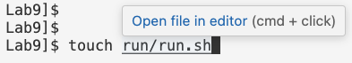
The main part of the VS Code window is the editor pane. Here, you can open text files and images. Create two new files:

touch run/run.sh scripts/nfc-rnaseq.sh

Then open the run.sh file in the editor – hold Ctrl/Cmd and click on the path in the command you just issued:

Or create and open files using the menus (Click to expand)

Open a new file: Click the hamburger menu , then File > New File.
Save the file (Ctrl/⌘+S), inside one of the dirs you just created: Lab9/run/run.sh.
Repeat steps 1 and 2 to create a file Lab9/scripts/nfc-rnaseq.sh.
Find the run.sh file in the File Explorer in the left side bar, and click on it to open.

Some VS Code tips and tricks (Click to expand)

A folder as a starting point
Conveniently, VS Code takes a specific directory as a starting point in all parts of the program:
- In the file explorer in the side bar
- In the terminal
- When saving files in the editor pane.
This is why your terminal was “already” located in /fs/scratch/PAS2658/<your-name>.
(If you need to switch folders, click > File > Open Folder.)
Resizing panes
You can resize panes (terminal, editor, side bar) by hovering your cursor over the borders and then dragging.
Hide the side bars
If you want to save some screen space while coding along in class, you may want to occasionally hide the side bars:
- In > View > Appearance you can toggle both the Activity Bar (narrow side bar) and the Primary Side Bar (wide side bar).
- Or use keyboard shortcuts:
  - Ctrl/⌘+B for the primary/wide side bar
  - Ctrl+Shift+B for the activity/narrow side bar
The Command Palette
To access all the menu options that are available in VS Code, the so-called “Command Palette” can be handy, especially if you know what you are looking for. To access the Command Palette, click and then Command Palette (or press F1 or Ctrl/⌘+Shift+P). To use it, start typing something to look for an option.
Keyboard shortcuts
For a single-page PDF overview of keyboard shortcuts for your operating system: => Help => Keyboard Shortcut Reference. (Or for direct links to these PDFs: Windows / Mac / Linux.)
Install the Shellcheck extension
Click the gear icon and then Extensions, and search for and then install the shellcheck (by simonwong) extension, which will check your shell scripts for errors, and is extremely useful.

3 Setting up

3.1 Getting your own copy of the data

As mentioned above, we will use the RNA-seq data from Garrigos et al. 2023. However, to keep things manageable for a lab like this, I have subset the data set we’ll be working with: I omitted the 21-day samples and only kept 500,000 reads per FASTQ file. All in all, our set of files consists of:

44 paired-end Illumina RNA-seq FASTQ files for 22 samples.
Culex pipiens reference genome files from NCBI: assembly in FASTA format and annotation in GTF format.
A metadata file in TSV format matching sample IDs with treatment & time point info.
A README file describing the data set.

Go ahead and get yourself a copy of the data with cp command:

# (Using the -r option for recursive copying, and -v to print what it's doing)
cp -rv /fs/scratch/PAS2658/jelmer/share/* .

‘/fs/scratch/PAS2658/jelmer/share/data’ -> ‘./data’
‘/fs/scratch/PAS2658/jelmer/share/data/meta’ -> ‘./data/meta’
‘/fs/scratch/PAS2658/jelmer/share/data/meta/metadata.tsv’ -> ‘./data/meta/metadata.tsv’
‘/fs/scratch/PAS2658/jelmer/share/data/ref’ -> ‘./data/ref’
‘/fs/scratch/PAS2658/jelmer/share/data/ref/GCF_016801865.2.gtf’ -> ‘./data/ref/GCF_016801865.2.gtf’
‘/fs/scratch/PAS2658/jelmer/share/data/ref/GCF_016801865.2.fna’ -> ‘./data/ref/GCF_016801865.2.fna’
‘/fs/scratch/PAS2658/jelmer/share/data/fastq’ -> ‘./data/fastq’
‘/fs/scratch/PAS2658/jelmer/share/data/fastq/ERR10802868_R2.fastq.gz’ -> ‘./data/fastq/ERR10802868_R2.fastq.gz’
‘/fs/scratch/PAS2658/jelmer/share/data/fastq/ERR10802863_R1.fastq.gz’ -> ‘./data/fastq/ERR10802863_R1.fastq.gz’
‘/fs/scratch/PAS2658/jelmer/share/data/fastq/ERR10802886_R2.fastq.gz’ -> ‘./data/fastq/ERR10802886_R2.fastq.gz’
# [...output truncated...]

Use the tree command to get a nice overview of the files you copied:

# '-C' will add colors to the output (not visible in the output below)
tree -C data

data
├── fastq
│   ├── ERR10802863_R1.fastq.gz
│   ├── ERR10802863_R2.fastq.gz
│   ├── ERR10802864_R1.fastq.gz
│   ├── ERR10802864_R2.fastq.gz
│   ├── ERR10802865_R1.fastq.gz
│   ├── ERR10802865_R2.fastq.gz
    ├── [...truncated...]
├── meta
│   └── metadata.tsv
├── README.md
└── ref
    ├── GCF_016801865.2.fna
    └── GCF_016801865.2.gtf

3 directories, 48 files

We’ll take a look at some of the files:

The metadata file:

cat data/meta/metadata.tsv

sample_id       time    treatment
ERR10802882     10dpi   cathemerium
ERR10802875     10dpi   cathemerium
ERR10802879     10dpi   cathemerium
ERR10802883     10dpi   cathemerium
ERR10802878     10dpi   control
ERR10802884     10dpi   control
ERR10802877     10dpi   control
ERR10802881     10dpi   control
ERR10802876     10dpi   relictum
ERR10802880     10dpi   relictum
ERR10802885     10dpi   relictum
ERR10802886     10dpi   relictum
ERR10802864     24hpi   cathemerium
ERR10802867     24hpi   cathemerium
ERR10802870     24hpi   cathemerium
ERR10802866     24hpi   control
ERR10802869     24hpi   control
ERR10802863     24hpi   control
ERR10802871     24hpi   relictum
ERR10802874     24hpi   relictum
ERR10802865     24hpi   relictum
ERR10802868     24hpi   relictum

The FASTQ files:

ls -lh data/fastq

total 941M
-rw-r--r-- 1 jelmer PAS2658 21M Mar 23 12:40 ERR10802863_R1.fastq.gz
-rw-r--r-- 1 jelmer PAS2658 22M Mar 23 12:40 ERR10802863_R2.fastq.gz
-rw-r--r-- 1 jelmer PAS2658 21M Mar 23 12:40 ERR10802864_R1.fastq.gz
-rw-r--r-- 1 jelmer PAS2658 22M Mar 23 12:40 ERR10802864_R2.fastq.gz
-rw-r--r-- 1 jelmer PAS2658 22M Mar 23 12:40 ERR10802865_R1.fastq.gz
-rw-r--r-- 1 jelmer PAS2658 22M Mar 23 12:40 ERR10802865_R2.fastq.gz
-rw-r--r-- 1 jelmer PAS2658 21M Mar 23 12:40 ERR10802866_R1.fastq.gz
-rw-r--r-- 1 jelmer PAS2658 22M Mar 23 12:40 ERR10802866_R2.fastq.gz
-rw-r--r-- 1 jelmer PAS2658 22M Mar 23 12:40 ERR10802867_R1.fastq.gz
-rw-r--r-- 1 jelmer PAS2658 22M Mar 23 12:40 ERR10802867_R2.fastq.gz
# [...output truncated...]

3.2 How we’ll run the pipeline

As discussed in the lecture, the entire nf-core rnaseq pipeline can be run with a single command. That said, before we can do so, we’ll need to a bunch of prep, such as:

Activating the software environment and downloading the pipeline files.
Defining the pipeline’s inputs and outputs, which includes creating a “sample sheet”.
Creating a small “config file” to run Nextflow pipelines at OSC.

We need the latter configuration because the pipeline will submit Slurm batch jobs for us for each step of the pipeline. And in most steps, programs are run independently for each sample, so the pipeline will submit a separate job for each sample for these steps — therefore, we’ll have many jobs altogether (typically 100s).

The main Nextflow process does not need much computing power (a single core with the default 4 GB of RAM will be sufficient) and even though our VS Code shell already runs on a compute and not a login node, we are still better off submitting the main process as a batch job as well, because:

This process can run for hours and we don’t want to risk it disconnecting.
We want to store all the standard output about pipeline progress and so on to a file — this will automatically end up in a Slurm log file if we submit it as a batch job.

3.3 Conceptual overview of our script setup

We will be working with two scripts in this lab, both of which you already created an empty file for:

A “runner” script that you can also think of as a digital lab notebook, containing commands that we run interactively.
A script that we will submit as a Slurm batch job with sbatch, containing code to run the nf-core nextflow pipeline.

To give you an idea of what this will look like — the runner script will include code like this, which will submit the job script:

# [Don't run or copy this]
sbatch scripts/nfc_rnaseq.sh "$samplesheet" "$fasta" "$gtf" "$outdir"

The variables above ("$samplesheet" etc.) are the inputs and outputs of the pipeline, which we will have defined elsewhere in the runner script. Inside the job script, we will then use these variables to run the pipeline in a specific way.

3.4 Activating the Conda environment

To save some time, you won’t do your own Conda installation of Nextflow or nf-core tools — I’ve installed both in an environment you can activate as follows:

# [Paste this code into the run/run.sh script, then run it in the terminal]

# First load OSC's (mini)Conda module
module load miniconda3
# Then activate the Nextflow conda environment 
source activate /fs/ess/PAS0471/jelmer/conda/nextflow

Check that Nextflow and nf-core tools can be run by printing the versions:

# [Run this code directly in the terminal]
nextflow -v

nextflow version 23.10.1.5891

# [Run this code directly in the terminal]
nf-core --version

                                          ,--./,-.
          ___     __   __   __   ___     /,-._.--~\
    |\ | |__  __ /  ` /  \ |__) |__         }  {
    | \| |       \__, \__/ |  \ |___     \`-._,-`-,
                                          `._,._,'

    nf-core/tools version 2.13.1 - https://nf-co.re

nf-core, version 2.13.1

3.5 Downloading the nf-core rnaseq pipeline

We’ll use the nf-core download command to download the rnaseq pipeline’s files.

First, we need to set the environment variable NXF_SINGULARITY_CACHEDIR to tell Nextflow where to store the Singularity containers for all the tools the pipeline runs¹. We will use a dir of mine that already has all containers, to save some downloading time²:

# [Paste this code into the run/run.sh script, then run it in the terminal]

# Create an environment variable for the container dir
export NXF_SINGULARITY_CACHEDIR=/fs/ess/PAS0471/containers

Next, we’ll run the nf-core download command to download the currently latest version (3.14.0) of the rnaseq pipeline to software/rnaseq, and the associated container files to the previously specified dir:

# [Paste this code into the run/run.sh script, then run it in the terminal]

# Download the nf-core rnaseq pipeline files
nf-core download rnaseq \
    --revision 3.14.0 \
    --outdir software/nfc-rnaseq \
    --compress none \
    --container-system singularity \
    --container-cache-utilisation amend \
    --download-configuration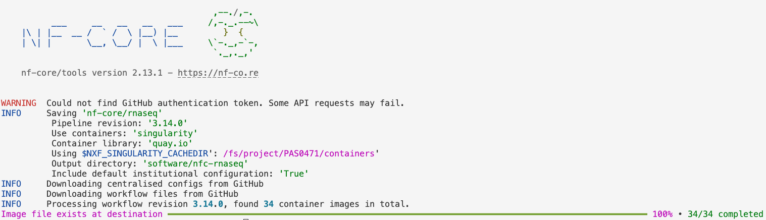

Explanation of all options given to nf-core download (Click to expand)

--revision: The version of the rnaseq pipeline.
--outdir: The dir to save the pipeline definition files.
--compress: Whether to compress the pipeline files — we chose not to.
--container-system: The type of containers to download. This should always be singularity at OSC, because that’s the only supported type.
--container-cache-utilisation: This is a little technical and not terribly interesting, but we used amend, which will make it check our $NXF_SINGULARITY_CACHEDIR dir for existing containers, and simply download any that aren’t already found there.
--download-configuration: This will download some configuration files that we will actually not use, but if you don’t provide this option, it will ask you about it when you run the command.

Also, don’t worry about the following warning, this doesn’t impact the downloading:

WARNING Could not find GitHub authentication token. Some API requests may fail.

Let’s take a quick peek at the dirs and files we just downloaded:

# [Run this code directly in the terminal]
ls software/nfc-rnaseq

3_14_0  configs

# [Run this code directly in the terminal]
ls software/nfc-rnaseq/3_14_0

assets        CODE_OF_CONDUCT.md  LICENSE       nextflow.config       subworkflows
bin           conf                main.nf       nextflow_schema.json  tower.yml
CHANGELOG.md  docs                modules       pyproject.toml        workflows
CITATIONS.md  lib                 modules.json  README.md

The dir and file structure here is unfortunately quite complicated, as are the individual pipeline definition files, so we won’t go into further detail about that here.

4 Writing a shell script to run the pipeline

In this section, we’ll go through the components of the scripts/nfc-rnaseq.sh script that we’ll later submit as a Slurm batch job. The most important part of this script is the nextflow command that will actually run the pipeline.

4.1 Building our `nextflow run` command

To run the pipeline, we use the command nextflow run, followed by the path to the dir that we just downloaded:

# [Partial shell script code, don't copy or run]
nextflow run software/nfc-rnaseq/3_14_0

After that, there are several required options (see the pipeline’s documentation), which represent the input and output files/dirs for the pipeline:

--input: The path to a “sample sheet” with the paths to FASTQ files (more on that below).
--fasta: The path to a reference genome assembly FASTA file — we’ll use the FASTA file we have in data/ref.
--gtf: The path to a reference genome annotation file³ — we’ll use the GTF file we have in data/ref.
--outdir: The path to the desired output dir for the final pipeline output — this can be whatever we like.

As discussed in the lecture, this pipeline has different options for e.g. alignment and quantification. We will stick close to the defaults, which includes alignment with STAR and quantification with Salmon, with one exception: we want to remove reads from ribosomal RNA (this step is skipped by default).

Exercise: Finding the option to remove rRNA

Take a look at the “Parameters” tab on the pipeline’s documentation website:

Browse through the options for a bit to get a feel for the extent to which you can customize the pipeline.
Try to find the option to turn on removal of rRNA with SortMeRNA.

Click for the solution

The option we want is --remove_ribo_rna.

We’ll also use several general Nextflow options (note the single dash - notation; pipeline-specific options have --):

-profile: A so-called “profile” — should be singularity when running the pipeline with Singularity containers.
work-dir: The dir in which all the pipeline’s jobs/processes will run.
-ansi-log false: Change Nextflow’s progress “logging” type to a format that works with Slurm log files⁴.
-resume: Resume the pipeline where it “needs to” (e.g., where it left off) instead of always starting over.

More on -work-dir and -resume (Click to expand)

work-dir:

The pipeline’s final outputs will go to the --outdir we talked about earlier. But all jobs/processes will run in, and initial outputs will be written to, a so-called -work-dir. After each process finishes, its key output files will then be copied to the final output dir. (There are also several pipeline options to customize what will and will not be copied.)

The distinction between such a work-dir and a final output dir can be very useful on HPC systems like OSC: you can use a scratch dir (at OSC: /fs/scratch/) with lots of storage space and fast I/O as the work-dir, and a backed-up project dir (at OSC: /fs/ess/) as the outdir, which will then not become unnecessarily large.

-resume:

Besides resuming wherever the pipeline left off after an incomplete run (for example: it ran out of time or ran into an error), the -resume option also checks for any changes in input files or pipeline settings.

For example, if you have run the pipeline to completion previously, but rerun it after adding or replace one sample, -resume would make the pipeline only rerun the “single-sample steps” of the pipeline (which is most of them) for that sample as well as all steps that use all samples. Similarly, if you change an option that affects one of the first processes in the pipeline, the entire pipeline may be rerun, whereas if you change an option that only affects the last process, then only that last process would be rerun.

This option won’t make any difference when we run the pipeline for the first time, since there is nothing to resume. Nextflow will even give a warning along these lines, but this is not a problem.

With all the above-mentioned options, our final nextflow run command will be:

# [Partial shell script code, don't copy or run]
nextflow run software/nfc-rnaseq/3_14_0 \
    --input "$samplesheet" \
    --fasta "$fasta" \
    --gtf "$gtf" \
    --outdir "$outdir" \
    --remove_ribo_rna \
    -work-dir "$outdir"/raw \
    -profile singularity \
    -ansi-log false \
    -resume

The command uses several variables (e.g. "$samplesheet") — these will enter the script via command-line arguments.

4.2 Creating an OSC configuration file

To speed things up and make use of the computing power at OSC, we want the pipeline to submit Slurm batch jobs for us.

We have to tell it to do this, and how, using a configuration (config) file. There are multiple ways of storing this file and telling Nextflow about it — the one we’ll use is to simply create a file nextflow.config in the dir from which we submit the nextflow run command: Nextflow will automatically detect and parse such a file.

We will keep this file as simple as possible, only providing the “executor” (in our case: the Slurm program) and the OSC project to use:

echo "
process.executor = 'slurm'
process.clusterOptions='--account=PAS2658'
" > nextflow.config

4.3 Adding `#SBATCH` options

We will use #SBATCH header lines to define some parameters for our batch job for Slurm. Note that these are only for the “main” Nextflow job, not for the jobs that Nextflow itself will submit!

#SBATCH --account=PAS2658
#SBATCH --time=3:00:00
#SBATCH --mail-type=END,FAIL
#SBATCH --output=slurm-nfc_rnaseq-%j.out

--account=PAS2658: As always, we have to specify the OSC project.
--time=3:00:00: Ask for 3 hours (note that for a run of a full data set, you may want to use 6-24 hours).
--mail-type=END,FAIL: Have Slurm send us an email when the job ends normally or with an error.
--output=slurm-nfc_rnaseq-%j.out: Use a descriptive Slurm log file name (%j is the Slurm job number).

We only a need a single core and up to a couple GB of RAM, so the associated Slurm defaults will work for us.

4.4 The final script

We’ve covered most of the pieces of our script. Below is the full code for the script, in which I also added:

A shebang header line to indicate that this is a Bash shell script: #!/bin/bash.
A line to use “strict Bash settings”, set -euo pipefail⁵.
Some echo reporting of arguments/variables, printing the date, etc.

Open your scripts/nfc-rnaseq.sh script and paste the following into it:

#!/bin/bash
#SBATCH --account=PAS2658
#SBATCH --time=3:00:00
#SBATCH --mail-type=END,FAIL
#SBATCH --output=slurm-nfc_rnaseq-%j.out

# Settings and constants
WORKFLOW_DIR=software/nfc-rnaseq/3_14_0

# Load the Nextflow Conda environment
module load miniconda3
source activate /fs/ess/PAS0471/jelmer/conda/nextflow
export NXF_SINGULARITY_CACHEDIR=/fs/ess/PAS0471/containers

# Strict Bash settings
set -euo pipefail

# Process command-line arguments
samplesheet=$1
fasta=$2
gtf=$3
outdir=$4

# Report
echo "Starting script nfc-rnaseq.sh"
date
echo "Samplesheet:          $samplesheet"
echo "Reference FASTA:      $fasta"
echo "Reference GTF:        $gtf"
echo "Output dir:           $outdir"
echo

# Create the output dir
mkdir -p "$outdir"

# Create the config file
echo "
process.executor = 'slurm'
process.clusterOptions='--account=PAS2658'
" > nextflow.config

# Run the workflow
nextflow run "$WORKFLOW_DIR" \
    --input "$samplesheet" \
    --fasta "$fasta" \
    --gtf "$gtf" \
    --outdir "$outdir" \
    --remove_ribo_rna \
    -work-dir "$outdir"/raw \
    -profile singularity \
    -ansi-log false \
    -resume

# Report
echo "Done with script nfc-rnaseq.sh"
date

Exercise: Take a look at the script

Go through your complete scripts/nfc-rnaseq.sh script and see if you understand everything that’s going on in there. Ask if you’re confused about anything!

5 Running the pipeline

We will now switch back to the run/run.sh script to add the code to submit our script. But we’ll have to create a sample sheet first.

5.1 Preparing the sample sheet

This pipeline requires a “sample sheet” as one of its inputs. In the sample sheet, you provide the paths to your FASTQ files and the so-called “strandedness” of your RNA-Seq library.

RNA-Seq library strandedness

During RNA-Seq library prep, information about the directionality of the original RNA transcripts can be retained (resulting in a “stranded” library) or lost (resulting in an “unstranded” library: specify unstranded in the sample sheet).

In turn, stranded libraries can prepared either in reverse-stranded (reverse, by far the most common) or forward-stranded (forward) fashion. For more information about library strandedness, see this page.

The pipeline also allows for a fourth option: auto, in which case the strandedness is automatically determined at the start of the pipeline by pseudo-mapping a small proportion of the data with Salmon.

The sample sheet should be a plain-text comma-separated values (CSV) file. Here is the example file from the pipeline’s documentation:

sample,fastq_1,fastq_2,strandedness
CONTROL_REP1,AEG588A1_S1_L002_R1_001.fastq.gz,AEG588A1_S1_L002_R2_001.fastq.gz,auto
CONTROL_REP1,AEG588A1_S1_L003_R1_001.fastq.gz,AEG588A1_S1_L003_R2_001.fastq.gz,auto
CONTROL_REP1,AEG588A1_S1_L004_R1_001.fastq.gz,AEG588A1_S1_L004_R2_001.fastq.gz,auto

So, we need a header row with column names, then one row per sample, and the following columns:

Sample ID (we will simply use the part of the file names shared by R1 and R2).
R1 FASTQ file path (including the dir unless they are in your working dir).
R2 FASTQ file path (idem).
Strandedness: unstranded, reverse, forward, or auto — this data is forward-stranded, so we’ll use forward.

You can create this file in several ways — we will do it here with a helper script that comes with the pipeline⁶:

First, we define an output dir (this will also be the output dir for the pipeline), and the sample sheet file name:

# [Paste this into run/run.sh and then run it in the terminal]

# Define the output dir and sample sheet file name
outdir=results/nfc-rnaseq
samplesheet="$outdir"/nfc_samplesheet.csv
mkdir -p "$outdir"

Next, we run that helper script, specifying the strandedness of our data, the suffices of the R1 and R2 FASTQ files, and as arguments at the end, the input FASTQ dir (data/fastq) and the output file ($samplesheet):

# [Paste this into run/run.sh and then run it in the terminal]

# Create the sample sheet for the nf-core pipeline
python3 software/nfc-rnaseq/3_14_0/bin/fastq_dir_to_samplesheet.py \
    --strandedness forward \
    --read1_extension "_R1.fastq.gz" \
    --read2_extension "_R2.fastq.gz" \
    data/fastq \
    "$samplesheet"

Finally, let’s check the contents of our newly created sample sheet file:

# [Run this directly in the terminal]
cat "$samplesheet"

sample,fastq_1,fastq_2,strandedness
ERR10802863,data/fastq/ERR10802863_R1.fastq.gz,data/fastq/ERR10802863_R2.fastq.gz,forward
ERR10802864,data/fastq/ERR10802864_R1.fastq.gz,data/fastq/ERR10802864_R2.fastq.gz,forward
ERR10802865,data/fastq/ERR10802865_R1.fastq.gz,data/fastq/ERR10802865_R2.fastq.gz,forward
ERR10802866,data/fastq/ERR10802866_R1.fastq.gz,data/fastq/ERR10802866_R2.fastq.gz,forward
ERR10802867,data/fastq/ERR10802867_R1.fastq.gz,data/fastq/ERR10802867_R2.fastq.gz,forward
ERR10802868,data/fastq/ERR10802868_R1.fastq.gz,data/fastq/ERR10802868_R2.fastq.gz,forward
ERR10802869,data/fastq/ERR10802869_R1.fastq.gz,data/fastq/ERR10802869_R2.fastq.gz,forward
ERR10802870,data/fastq/ERR10802870_R1.fastq.gz,data/fastq/ERR10802870_R2.fastq.gz,forward
ERR10802871,data/fastq/ERR10802871_R1.fastq.gz,data/fastq/ERR10802871_R2.fastq.gz,forward
ERR10802874,data/fastq/ERR10802874_R1.fastq.gz,data/fastq/ERR10802874_R2.fastq.gz,forward
ERR10802875,data/fastq/ERR10802875_R1.fastq.gz,data/fastq/ERR10802875_R2.fastq.gz,forward
ERR10802876,data/fastq/ERR10802876_R1.fastq.gz,data/fastq/ERR10802876_R2.fastq.gz,forward
ERR10802877,data/fastq/ERR10802877_R1.fastq.gz,data/fastq/ERR10802877_R2.fastq.gz,forward
ERR10802878,data/fastq/ERR10802878_R1.fastq.gz,data/fastq/ERR10802878_R2.fastq.gz,forward
ERR10802879,data/fastq/ERR10802879_R1.fastq.gz,data/fastq/ERR10802879_R2.fastq.gz,forward
ERR10802880,data/fastq/ERR10802880_R1.fastq.gz,data/fastq/ERR10802880_R2.fastq.gz,forward
ERR10802881,data/fastq/ERR10802881_R1.fastq.gz,data/fastq/ERR10802881_R2.fastq.gz,forward
ERR10802882,data/fastq/ERR10802882_R1.fastq.gz,data/fastq/ERR10802882_R2.fastq.gz,forward
ERR10802883,data/fastq/ERR10802883_R1.fastq.gz,data/fastq/ERR10802883_R2.fastq.gz,forward
ERR10802884,data/fastq/ERR10802884_R1.fastq.gz,data/fastq/ERR10802884_R2.fastq.gz,forward
ERR10802885,data/fastq/ERR10802885_R1.fastq.gz,data/fastq/ERR10802885_R2.fastq.gz,forward
ERR10802886,data/fastq/ERR10802886_R1.fastq.gz,data/fastq/ERR10802886_R2.fastq.gz,forward

Creating the sample sheet with shell commands instead (Click to expand)

# A) Define the file name and create the header line
echo "sample,fastq_1,fastq_2,strandedness" > "$samplesheet"
  
# B) Add a row for each sample based on the file names
ls data/fastq/* | paste -d, - - |
    sed -E -e 's/$/,forward/' -e 's@.*/(.*)_R1@\1,&@' >> "$samplesheet"

Here is an explanation of the last command:

The ls command will spit out a list of all FASTQ files that includes the dir name.
paste - - will paste that FASTQ files side-by-side in two columns — because there are 2 FASTQ files per sample, and they are automatically correctly ordered due to their file names, this will create one row per sample with the R1 and R2 FASTQ files next to each other.
The -d, option to paste will use a comma instead of a Tab to delimit columns.
We use sed with extended regular expressions (-E) and two separate search-and-replace expressions (we need -e in front of each when there is more than one).
The first sed expression 's/$/,forward/' will simply add ,forward at the end ($) of each line to indicate the strandedness.
The second sed expression, 's@.*/(.*)_R1@\1,&@':
- Here we are adding the sample ID column by copying that part from the R1 FASTQ file name.
- This uses s@<search>@replace@ with @ instead of /, because there is a / in our search pattern.
- In the search pattern (.*/(.*)_R1), we capture the sample ID with (.*).
- In the replace section (\1,&), we recall the captured sample ID with \1, then insert a comma, and then insert the full search pattern match (i.e., the path to the R1 file) with &.
We append (>>) to the file because we need to keep the header line that we had already put in it.

5.2 Submitting our shell script

As a last preparatory step, we will save the paths of the reference genome files in variables:

# [Paste this into run/run.sh and then run it in the terminal]
# Define the reference genome files
fasta=data/ref/GCF_016801865.2.fna
gtf=data/ref/GCF_016801865.2.gtf

Before we submit the script, let’s check that all the variables have been assigned by prefacing the command with echo:

# [ Run this directly in the terminal]
echo sbatch scripts/nfc-rnaseq.sh "$samplesheet" "$fasta" "$gtf" "$outdir"

sbatch scripts/nfc-rnaseq.sh results/nfc-rnaseq/nfc_samplesheet.csv data/ref/GCF_016801865.2.fna data/ref/GCF_016801865.2.gtf results/nfc-rnaseq

Now we are ready to submit the script as a batch job:

# [Paste this into run/run.sh and then run it in the terminal]
# Submit the script to run the pipeline as a batch job
sbatch scripts/nfc-rnaseq.sh "$samplesheet" "$fasta" "$gtf" "$outdir"

Submitted batch job 27767854

5.3 Checking the pipeline’s progress

We can check whether our job has started running, and whether Nextflow has already spawned jobs, with squeue:

# [Run this directly in the terminal]
squeue -u $USER -l

Mon Mar 25 12:13:38 2024
      JOBID PARTITION     NAME     USER    STATE   TIME TIME_LIMI  NODES NODELIST(REASON)
  27767854 serial-40 nfc-rnas   jelmer  RUNNING    1:33   3:00:00      1 p0219

In the example output above, the only running job is the one we directly submitted, i.e. the main Nextflow process. Because we didn’t give the job a name, the NAME column is the script’s name, nfc-rnaseq.sh (truncated to nfc-rnas).

See examples of squeue output that includes Nextflow-submitted jobs (Click to expand)

The top job, with partial name nf-NFCOR, is a job that’s been submitted by Nextflow:

squeue -u $USER -l

Mon Mar 25 13:14:53 2024
             JOBID PARTITION     NAME     USER    STATE       TIME TIME_LIMI  NODES NODELIST(REASON)
          27767861 serial-40 nf-NFCOR   jelmer  RUNNING       5:41  16:00:00      1 p0053
          27767854 serial-40 nfc_rnas   jelmer  RUNNING    1:03:48   3:00:00      1 p0219

Unfortunately, the columns in the output above are quite narrow, so it’s not possible to see which step of the pipeline is being run by that job. The following (awful-looking!) code can be used to make that column much wider, so we can see the job’s full name which makes clear which step is being run (rRNA removal with SortMeRNA):

squeue -u $USER --format="%.9i %.9P %.60j %.8T %.10M %.10l %.4C %R %.16V"

Mon Mar 25 13:15:05 2024
    JOBID PARTITION                                                          NAME    STATE       TIME TIME_LIMIT CPUS NODELIST(REASON)      SUBMIT_TIME
 27767861 serial-40   nf-NFCORE_RNASEQ_RNASEQ_SORTMERNA_(SRR27866691_SRR27866691)  RUNNING       5:55   16:00:00   12 p0053 2024-03-23T09:37
 27767854 serial-40                                                    nfc_rnaseq  RUNNING    1:04:02    3:00:00    1 p0219 2024-03-23T09:36

You might also catch the pipeline while there are many more jobs running, e.g.:

Mon Mar 25 13:59:50 2024
             JOBID PARTITION     NAME     USER    STATE       TIME TIME_LIMI  NODES NODELIST(REASON)
          27823107 serial-40 nf-NFCOR   jelmer  RUNNING       0:13  16:00:00      1 p0091
          27823112 serial-40 nf-NFCOR   jelmer  RUNNING       0:13  16:00:00      1 p0119
          27823115 serial-40 nf-NFCOR   jelmer  RUNNING       0:13  16:00:00      1 p0055
          27823120 serial-40 nf-NFCOR   jelmer  RUNNING       0:13  16:00:00      1 p0055
          27823070 serial-40 nf-NFCOR   jelmer  RUNNING       0:43  16:00:00      1 p0078
          27823004 serial-40 nfc-rnas   jelmer  RUNNING       2:13   3:00:00      1 p0146
          27823083 serial-40 nf-NFCOR   jelmer  RUNNING       0:37  16:00:00      1 p0078
          27823084 serial-40 nf-NFCOR   jelmer  RUNNING       0:37  16:00:00      1 p0096
          27823085 serial-40 nf-NFCOR   jelmer  RUNNING       0:37  16:00:00      1 p0096
          27823086 serial-40 nf-NFCOR   jelmer  RUNNING       0:37  16:00:00      1 p0115
          27823087 serial-40 nf-NFCOR   jelmer  RUNNING       0:37  16:00:00      1 p0115
          27823088 serial-40 nf-NFCOR   jelmer  RUNNING       0:37  16:00:00      1 p0123
          27823089 serial-40 nf-NFCOR   jelmer  RUNNING       0:37  16:00:00      1 p0123
          27823090 serial-40 nf-NFCOR   jelmer  RUNNING       0:37  16:00:00      1 p0057
          27823091 serial-40 nf-NFCOR   jelmer  RUNNING       0:37  16:00:00      1 p0057
          27823092 serial-40 nf-NFCOR   jelmer  RUNNING       0:37  16:00:00      1 p0058
          27823093 serial-40 nf-NFCOR   jelmer  RUNNING       0:37  16:00:00      1 p0058
          27823095 serial-40 nf-NFCOR   jelmer  RUNNING       0:37  16:00:00      1 p0118
          27823099 serial-40 nf-NFCOR   jelmer  RUNNING       0:37  16:00:00      1 p0118
          27823103 serial-40 nf-NFCOR   jelmer  RUNNING       0:37  16:00:00      1 p0119
          27823121 serial-48 nf-NFCOR   jelmer  RUNNING       0:13  16:00:00      1 p0625
          27823122 serial-48 nf-NFCOR   jelmer  RUNNING       0:13  16:00:00      1 p0744
          27823123 serial-48 nf-NFCOR   jelmer  RUNNING       0:13  16:00:00      1 p0780
          27823124 serial-48 nf-NFCOR   jelmer  RUNNING       0:13  16:00:00      1 p0780

We can keep an eye on the pipeline’s progress, and see if there are any errors, by checking the Slurm log file — the top of the file should look like this:

# You will have a different job ID - replace as appropriate or use Tab completion
less slurm-nfc_rnaseq-27767861.out

Starting script nfc-rnaseq.sh
Mon Mar 25 13:01:30 EDT 2024
Samplesheet:          results/nfc-rnaseq/nfc_samplesheet.csv
Reference FASTA:      data/ref/GCF_016801865.2.fna
Reference GTF:        data/ref/GCF_016801865.2.gtf
Output dir:           results/nfc-rnaseq

N E X T F L O W  ~  version 23.10.1
WARN: It appears you have never run this project before -- Option `-resume` is ignored
Launching `software/nfc-rnaseq/3_14_0/main.nf` [curious_linnaeus] DSL2 - revision: 746820de9b
WARN: ~~~~~~~~~~~~~~~~~~~~~~~~~~~~~~~~~~~~~~~~~~~~~~~~~~~~~~~~~~~~~~~~~~~~~~
  Multiple config files detected!
  Please provide pipeline parameters via the CLI or Nextflow '-params-file' option.
  Custom config files including those provided by the '-c' Nextflow option can be
  used to provide any configuration except for parameters.

  Docs: https://nf-co.re/usage/configuration#custom-configuration-files
~~~~~~~~~~~~~~~~~~~~~~~~~~~~~~~~~~~~~~~~~~~~~~~~~~~~~~~~~~~~~~~~~~~~~~~~~~~~


------------------------------------------------------
                                        ,--./,-.
        ___     __   __   __   ___     /,-._.--~'
  |\ | |__  __ /  ` /  \ |__) |__         }  {
  | \| |       \__, \__/ |  \ |___     \`-._,-`-,
                                        `._,._,'
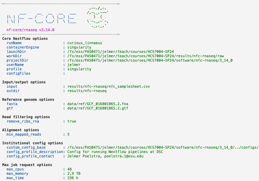
  nf-core/rnaseq v3.14.0
------------------------------------------------------
Core Nextflow options
  runName                   : curious_linnaeus
  containerEngine           : singularity
[...output truncated...]

The warnings about -resume and config files shown above can be ignored. Some of this output actually has nice colors:

In the Slurm log file, the job progress is show in the following way — we only see which jobs are being submitted, not when they finish⁷:

[e5/da8328] Submitted process > NFCORE_RNASEQ:RNASEQ:PREPARE_GENOME:GTF_FILTER (GCF_016801865.2.fna)
[b5/9427a1] Submitted process > NFCORE_RNASEQ:RNASEQ:PREPARE_GENOME:CUSTOM_GETCHROMSIZES (GCF_016801865.2.fna)
[05/e0e09f] Submitted process > NFCORE_RNASEQ:RNASEQ:FASTQ_FASTQC_UMITOOLS_TRIMGALORE:TRIMGALORE (ERR10802863)
[25/a6c2f5] Submitted process > NFCORE_RNASEQ:RNASEQ:FASTQ_FASTQC_UMITOOLS_TRIMGALORE:FASTQC (ERR10802863)
[24/cef9a0] Submitted process > NFCORE_RNASEQ:RNASEQ:FASTQ_FASTQC_UMITOOLS_TRIMGALORE:TRIMGALORE (ERR10802864)
[b1/9cfa7e] Submitted process > NFCORE_RNASEQ:RNASEQ:FASTQ_FASTQC_UMITOOLS_TRIMGALORE:FASTQC (ERR10802864)
[c4/3107c1] Submitted process > NFCORE_RNASEQ:RNASEQ:FASTQ_FASTQC_UMITOOLS_TRIMGALORE:TRIMGALORE (ERR10802865)
[7e/92ec89] Submitted process > NFCORE_RNASEQ:RNASEQ:FASTQ_FASTQC_UMITOOLS_TRIMGALORE:TRIMGALORE (ERR10802866)
[01/f7ccfb] Submitted process > NFCORE_RNASEQ:RNASEQ:FASTQ_FASTQC_UMITOOLS_TRIMGALORE:FASTQC (ERR10802866)
[42/4b4da2] Submitted process > NFCORE_RNASEQ:RNASEQ:FASTQ_FASTQC_UMITOOLS_TRIMGALORE:TRIMGALORE (ERR10802868)
[8c/fe6ca5] Submitted process > NFCORE_RNASEQ:RNASEQ:FASTQ_FASTQC_UMITOOLS_TRIMGALORE:TRIMGALORE (ERR10802867)
[e6/a12ec8] Submitted process > NFCORE_RNASEQ:RNASEQ:FASTQ_FASTQC_UMITOOLS_TRIMGALORE:FASTQC (ERR10802867)
[2e/f9059d] Submitted process > NFCORE_RNASEQ:RNASEQ:FASTQ_FASTQC_UMITOOLS_TRIMGALORE:FASTQC (ERR10802865)
[de/2735d1] Submitted process > NFCORE_RNASEQ:RNASEQ:FASTQ_FASTQC_UMITOOLS_TRIMGALORE:FASTQC (ERR10802868)

You should also see the following warning among the job submissions (Click to expand)

This warning can be ignored, the “Biotype QC” is not important and this information is indeed simply missing from our GTF file, there is nothing we can do about that.

WARN: ~~~~~~~~~~~~~~~~~~~~~~~~~~~~~~~~~~~~~~~~~~~~~~~~~~~~~~~~~~~~~~~~~~~~~~
  Biotype attribute 'gene_biotype' not found in the last column of the GTF file!

  Biotype QC will be skipped to circumvent the issue below:
  https://github.com/nf-core/rnaseq/issues/460

  Amend '--featurecounts_group_type' to change this behaviour.
~~~~~~~~~~~~~~~~~~~~~~~~~~~~~~~~~~~~~~~~~~~~~~~~~~~~~~~~~~~~~~~~~~~~~~~~~~~~

But any errors would be reported in this file, and we can also see when the pipeline has finished:

[28/79e801] Submitted process > NFCORE_RNASEQ:RNASEQ:BEDGRAPH_BEDCLIP_BEDGRAPHTOBIGWIG_FORWARD:UCSC_BEDGRAPHTOBIGWIG (ERR10802864)
[e0/ba48c9] Submitted process > NFCORE_RNASEQ:RNASEQ:BEDGRAPH_BEDCLIP_BEDGRAPHTOBIGWIG_REVERSE:UCSC_BEDGRAPHTOBIGWIG (ERR10802864)
[62/4f8c0d] Submitted process > NFCORE_RNASEQ:RNASEQ:MULTIQC (1)
-[nf-core/rnaseq] Pipeline completed successfully -
Done with script nfc-rnaseq.sh
Mon Mar 25 14:09:52 EDT 2024

6 Checking the pipeline’s outputs

If your pipeline run finished in time (it may finish in as little as 15-30 minutes, but this can vary substantially⁸), you can take a look at the files and dirs in the output dir we specified:

ls -lh results/nfc-rnaseq

total 83K
drwxr-xr-x   2 jelmer PAS0471  16K Mar 25 13:02 fastqc
drwxr-xr-x   2 jelmer PAS0471 4.0K Mar 25 12:58 logs
drwxr-xr-x   3 jelmer PAS0471 4.0K Mar 25 13:14 multiqc
-rw-r--r--   1 jelmer PAS0471 2.0K Mar 25 19:55 nfc_samplesheet.csv
drwxr-xr-x   2 jelmer PAS0471 4.0K Mar 25 13:14 pipeline_info
drwxr-xr-x 248 jelmer PAS0471  16K Mar 25 13:10 raw
drwxr-xr-x   2 jelmer PAS0471 4.0K Mar 25 13:06 sortmerna
drwxr-xr-x  33 jelmer PAS0471  16K Mar 25 13:12 star_salmon
drwxr-xr-x   3 jelmer PAS0471 4.0K Mar 25 13:02 trimgalore

The two outputs we are most interested in are:

The MultiQC report (<outdir>/multiqc/star_salmon/multiqc_report.html): this has lots of QC summaries of the data, both the raw data and the alignments, and even a gene expression PCA plot.
The gene count table (<outdir>/star_salmon/salmon.merged.gene_counts_length_scaled.tsv): if you do the Gene count table analysis lab, you will use an equivalent file (but then run on the full data set) as the main input.

6.1 The MultiQC report

You can find a copy of the MultiQC report on this website, here. Go ahead and open that in a separate browser tab. There’s a lot of information in the report! Here are some items to especially pay attention to, with figures from our own data set:

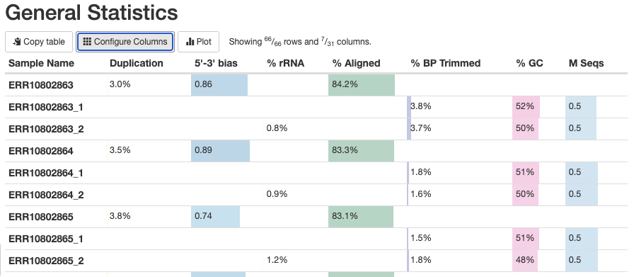
The General Statistics table (the first section) is very useful, with the following notes:
- Most of the table’s content is also in later graphs, but the table allows for comparisons across metrics.
- The %rRNA (% of reads identified as rRNA and removed by SortMeRNA) can only be found in this table.
- It’s best to hide the columns with statistics from Samtools, which can be confusing if not downright misleading: click on “Configure Columns” and uncheck all the boxes for stats with Samtools in their name.
- Some stats are for R1 and R2 files only, and some are for each sample as a whole. Unfortunately, this means you get 3 rows per sample in the table.

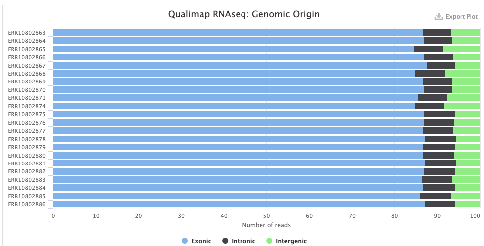
The Qualimap > Genomic origin of reads plot shows, for each sample, the proportion of reads mapping to exonic vs. intronic vs. intergenic regions. This is an important QC plot: the vast majority of your reads should be exonic⁹.

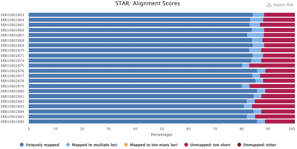
This is a good result, with 80-90% of mapped reads in exonic regions.

The STAR > Alignment Scores plot shows, for each sample, the percentage of reads that was mapped. Note that “Mapped to multiple loci” reads are also included in the final counts, and that “Unmapped: too short” merely means unmapped, really, and not that the reads were too short.

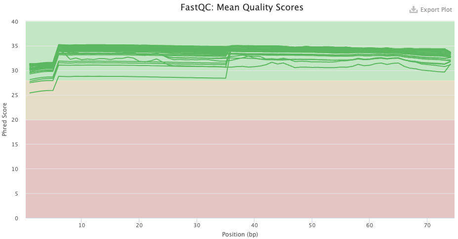
This is a pretty good results, with 80-90% of reads mapped.

FastQC checks your FASTQ files, i.e. your data prior to alignment. There are FastQC plots both before and after trimming with TrimGalore/Cutadapt. The most important FastQC modules are:
- Sequence Quality Histograms — You’d like the mean qualities to stay in the “green area”.
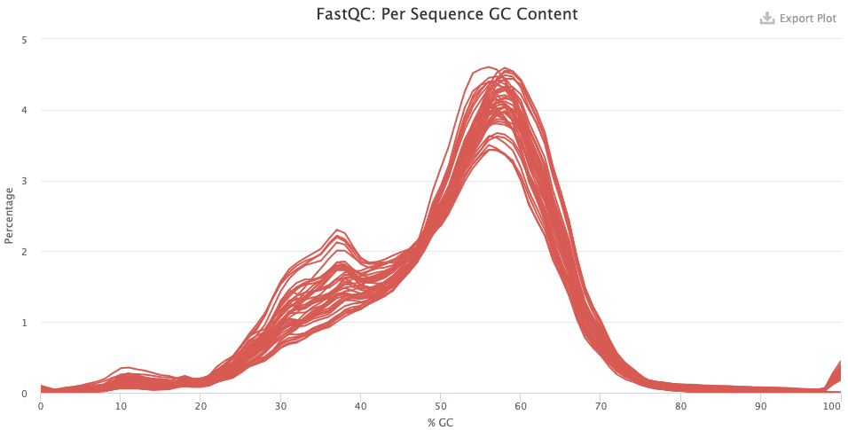
- Per Sequence GC Content — Secondary peaks may indicate contamination.
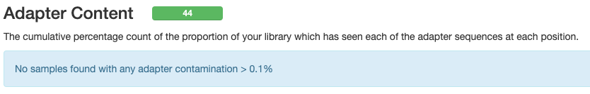
- Adapter Content — Any adapter content should be gone in the post-trimming plot.

Exercise: Interpreting FastQC results in the MultiQC report

Take a look at the three FastQC modules discussed above, both before and after trimming.

Has the base quality improved after trimming, and does this look good?

Click to see the answer

Pre-trimming graph: The qualities are good overall, but there is more variation that what is usual, and note the poorer qualities in the first 7 or so bases. There is no substantial decline towards the end of the read as one often sees with Illumina data, but this is expected given that the reads are only 75 bp.

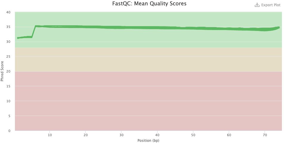
**Pre-trimming** (Mean base quality scores: one line is one sample.)

Post-trimming graph: The qualities have clearly improved. The first 7 or so bases remain of clearly poorer quality, on average.

Do you have any idea what’s going with the pre-trimming GC content distribution? What about after trimming — does this look good or is there reason to worry?

Click to see the answer

The pre-trimming GC content is very odd but this is mostly due to a high number of reads with zero and near-zero percent GC content. These are likely reads with only Ns. There are also some reads with near-hundred percent GC content. These are likely artifactual G-only reads that NextSeq/NovaSeq machines can produce.

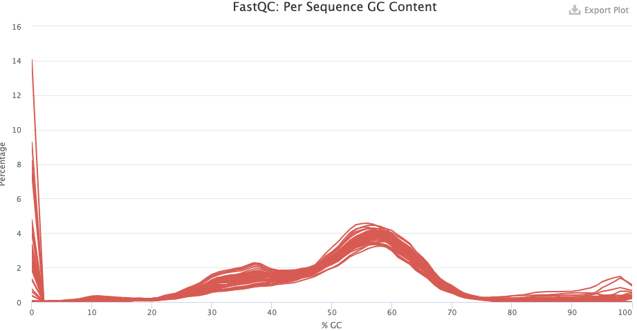
After trimming, things look a lot better but there may be contamination here, given the weird “shoulder” at 30-40% GC.

Do you know what the “adapters” that FastQC found pre-trimming are? Were these sequences removed by the trimming?

Click to see the answer

Pre-trimming, there seem to be some samples with very high adapter content throughout the read. This doesn’t make sense for true adapters, because these are usually only found towards the end of the read, when the read length is longer than the DNA fragment length. If you hover over the lines, you’ll see it says “polyg”. These are artifactual G-only reads that NextSeq/NovaSeq can produce, especially in the reverse reads — and you can see that all of the lines are for reverse-read files indeed.

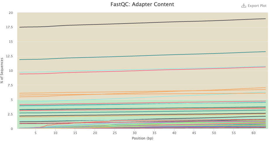
Post-trimming, no adapter content was found.

Some additional graphs of interest in the MultiQC report (Click to expand)

The Qualimap > Gene Coverage Profile plot. This shows average read-depth across the position of genes/transcripts (for all genes together), which helps to assess the amount of RNA degradation. For poly-A selected libraries, RNA molecules “begin” at the 3’ end (right-hand side of the graph), so the more degradation there is, the more you expect there to be a higher read-depth towards the 3’ end compared to the 5’ end. (Though note that sharp decreases at the very end on each side are expected.)

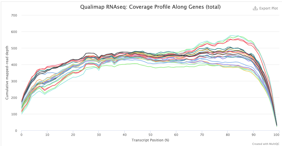
There depth at ~20% (near the 5’ end) is clearly lower than at ~80% (near the 3’ end),
indicating some RNA degradation.

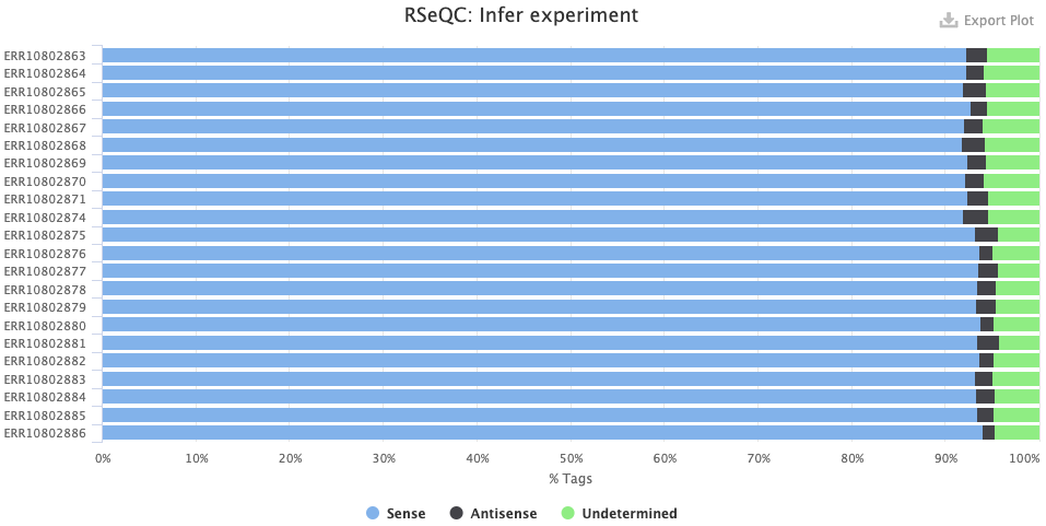
The RSeqQC > Infer experiment (library strandedness) plot. If your library is:
- Unstranded, there should be similar percentages of Sense and Antisense reads.
- Forward-stranded, the vast majority of reads should be Sense.
- Reverse-stranded, the vast majority of reads should be Antisense.

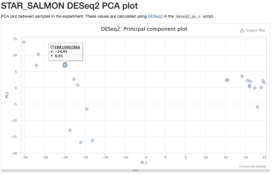
This libary is clearly forward-stranded, as we indicated in our sample sheet.

The STAR_SALMON DESeq2 PCA plot is from a Principal Component Analysis (PCA) run on the final gene count table, thus showing overall patterns of gene expression similarity among samples.

The sampels clear form two distinct groups along PC1.

Did your pipeline run finish? Here’s how to check out your own MultiQC report (Click to expand)

To download the MultiQC HTML file at results/nfc-rnaseq/multiqc/star_salmon/multiqc_report.html, find this file in the VS Code explorer (file browser) on the left, right-click on it, and select Download....

You can download it to any location on your computer. Then find the file on your computer and click on it to open it — it should be opened in your browser.

6.2 The gene count table

The gene count table has one row for each gene and one column for each sample, with the first two columns being the gene_id and gene_name¹⁰. Each cell’s value contains the read count estimate for a specific gene in a specific sample:

# [Paste this into the run/run.sh script and run it in the terminal]

# Take a look at the count table:
# ('column -t' lines up columns, and less's '-S' option turns off line wrapping)
counts=results/nfc-rnaseq/star_salmon/salmon.merged.gene_counts_length_scaled.tsv
column -t "$counts" | less -S

gene_id             gene_name           ERR10802863        ERR10802864        ERR10802865        ERR10802866        ERR10802867        ERR10802868       
ATP6                ATP6                163.611027228009   178.19903533081    82.1025390726658   307.649552934133   225.78249209207    171.251589309856  
ATP8                ATP8                0                  1.01047333891691   0                  0                  0                  0                 
COX1                COX1                1429.24769032452   2202.82009602881   764.584344577622   2273.6965332904    2784.47391614249   2000.51277019854  
COX2                COX2                116.537361366535   175.137972566817   54.0166352459629   256.592955351283   193.291937038438   164.125833130119  
COX3                COX3                872.88670991359    1178.29247734231   683.167933227141   1200.01735304529   1300.3853323715    1229.11746824104  
CYTB                CYTB                646.028108528182   968.256051104547   529.393909319439   1025.23768317788   1201.46662840336   842.533209911258  
LOC120412322        LOC120412322        0                  0                  0                  0                  0.995135178345792  0.996805450081561 
LOC120412324        LOC120412324        37.8326244586681   20.9489661184365   27.6702324729125   48.6417838830061   22.8313729348804   36.87899862428    
LOC120412325        LOC120412325        3.21074365394071   2.10702898851342   4.40315394778926   5.47978997387391   4.33241716734803   4.23386924919438  
LOC120412326        LOC120412326        0                  0                  0                  0                  0                  0                 
LOC120412327        LOC120412327        37.8206758601034   35.9063291323018   38.517771617566    27.7802608986967   37.6979028802121   32.885944667709   
LOC120412328        LOC120412328        35.0080600370267   20.0019192467143   23.9260736995594   30.0191332346116   21.0383665366408   28.9844776623531  
LOC120412329        LOC120412329        121.777922287929   112.794544755113   131.434181046282   127.753086659103   114.864750589664   131.589608063253  
LOC120412330        LOC120412330        42.8505448763697   28.9442284428204   36.6285174684674   46.7310765909945   42.7633834468768   26.9265243413636  
LOC120412331        LOC120412331        11.013179311581    9.00559907892481   12.9836833055803   13.029954361225    7.02624958751718   16.000552787954   
LOC120412332        LOC120412332        12.1055360835441   26.1231316926989   21.2767913384733   18.2783703626438   26.4932540325187   22.098808637857   
LOC120412333        LOC120412333        19.1159998132169   17.0558058070299   12.0965688236319   14.1510477997588   15.2033452089903   9.02624985028677  
LOC120412334        LOC120412334        9.01332125155807   3.00232591636489   5.99566364212933   11.0306919231504   8.03448732510427   11.0022053123759  
# [...output truncated...]

Count table versions

The workflow outputs several versions of the count table¹¹, but the one with gene_counts_length_scaled is the one we want:

gene_counts as opposed to transcript_counts for counts that are summed across transcripts for each gene.
length for estimates that have been adjusted to account for between-sample differences in mean transcript length (longer transcripts would be expected to produce more reads in sequencing).
scaled for estimates that have been scaled back using the “library sizes”, per-sample total read counts.

Footnotes

These kinds of settings are more commonly specified with command options, but somewhat oddly, this is the only way we can specify that here.↩︎
But if you want to run a pipeline yourself for your own research, make sure to use a dir that you have permissions to write to.↩︎
Preferably in GTF (.gtf) format, but the pipeline can accept GFF/GFF3 (.gff/.gff3) format files as well.↩︎
The default logging does not work well the output goes to a text file, as it will in our case because we will submit the script with the Nextflow command as a Slurm batch job.↩︎
These setting will make the script abort whenever an error occurs, and it will also turn referencing unassigned/non-existing variables into an error. This is a recommended best-practice line to include in all shell scripts.↩︎
The box below shows an alternative method with Unix shell commands↩︎
The default Nextflow logging (without -ansi-log false) does show when jobs finish, but this would result in very messy output in a Slurm log file.↩︎
This variation is mostly the result of variation in Slurm queue-ing times. The pipeline makes quite large resource requests, so you sometimes have to wait for a while for some jobs to start.↩︎
A lot of intronic content may indicate that you have a lot of pre-mRNA in your data; this is more common when your library prep used rRNA depletion instead of poly-A selection. A lot of intergenic content may indicate DNA contamination. Poor genome annotation quality may also contribute to a low percentage of exonic reads. The RSeQC > Read Distribution plot will show this with even more categories, e.g. separately showing UTRs.↩︎
Which happen to be the same here, but these are usually different.↩︎
And each version in two formats: .rds (a binary R object file type) and .tsv.↩︎

1 Introduction

2 Getting started with VS Code

2.1 Starting VS Code at OSC

2.2 The VS Code User Interface

Side bars

Terminal

Editor pane and Welcome document

3 Setting up

3.1 Getting your own copy of the data

3.2 How we’ll run the pipeline

3.3 Conceptual overview of our script setup

3.4 Activating the Conda environment

3.5 Downloading the nf-core rnaseq pipeline

4 Writing a shell script to run the pipeline

4.1 Building our nextflow run command

Exercise: Finding the option to remove rRNA

4.2 Creating an OSC configuration file

4.3 Adding #SBATCH options

4.4 The final script

Exercise: Take a look at the script

5 Running the pipeline

5.1 Preparing the sample sheet

5.2 Submitting our shell script

5.3 Checking the pipeline’s progress

6 Checking the pipeline’s outputs

6.1 The MultiQC report

Exercise: Interpreting FastQC results in the MultiQC report

6.2 The gene count table

Footnotes

Editor pane and `Welcome` document

4.1 Building our `nextflow run` command

4.3 Adding `#SBATCH` options