RNA-seq data files

Author

Jelmer Poelstra

Published

January 26, 2025

1 Introduction

1.1 Our dataset

We will work with RNA-seq data from the paper “Two avian Plasmodium species trigger different transcriptional responses on their vector Culex pipiens”, published in 2023 in Molecular Ecology (link):

This paper uses RNA-seq data to study gene expression in Culex pipiens mosquitos infected with malaria-causing Plasmodium protozoans — specifically, it compares mosquitos according to:

Infection status: Plasmodium cathemerium vs. P. relictum vs. control
Time after infection: 24 h vs. 10 days vs. 21 days

1.2 What we will do

Today we’ll focus on the general aspects of reference genomes and HTS data — specifically, we will:

See how you can find a reference genome and the associated files
Explore the reference genome files
Explore our HTS reads
Perform quality-control on some of our reads with a command-line tool, FastQC

Next week, after covering RNA-seq methodology in the lecture, we will run a differential expression analysis.

1.3 Getting your own copy of the files

The main data files in a reference-based HTS project are reference genome files and sequence reads. We’ll discuss those files in more detail below — first, let’s get everyone their own copy of the data.

Go to your personal dir in /fs/scratch/PAS2250/ENT6703:

# Replace `jelmer` with your personal dir's name!
cd /fs/scratch/PAS2250/ENT6703/jelmer

Then, use the Unix copy command cp as follows (yes, there’s a space + period at the end!):

cp -rv ../share/data .

‘/fs/scratch/PAS2250/ENT6703/share/data’ -> ‘./data’
‘/fs/scratch/PAS2250/ENT6703/share/data/meta’ -> ‘./data/meta’
‘/fs/scratch/PAS2250/ENT6703/share/data/meta/metadata.tsv’ -> ‘./data/meta/metadata.tsv’
‘/fs/scratch/PAS2250/ENT6703/share/data/ref’ -> ‘./data/ref’
‘/fs/scratch/PAS2250/ENT6703/share/data/ref/GCF_016801865.2.gtf’ -> ‘./data/ref/GCF_016801865.2.gtf’
‘/fs/scratch/PAS2250/ENT6703/share/data/ref/GCF_016801865.2.fna’ -> ‘./data/ref/GCF_016801865.2.fna’
‘/fs/scratch/PAS2250/ENT6703/share/data/fastq’ -> ‘./data/fastq’
‘/fs/scratch/PAS2250/ENT6703/share/data/fastq/ERR10802868_R2.fastq.gz’ -> ‘./data/fastq/ERR10802868_R2.fastq.gz’
‘/fs/scratch/PAS2250/ENT6703/share/data/fastq/ERR10802863_R1.fastq.gz’ -> ‘./data/fastq/ERR10802863_R1.fastq.gz’
‘/fs/scratch/PAS2250/ENT6703/share/data/fastq/ERR10802880_R2.fastq.gz’ -> ‘./data/fastq/ERR10802880_R2.fastq.gz’
‘/fs/scratch/PAS2250/ENT6703/share/data/fastq/ERR10802880_R1.fastq.gz’ -> ‘./data/fastq/ERR10802880_R1.fastq.gz’
# [...truncated...]

In the command above:

Option -r will enable “recursive” (=dirs, not just files) copying
Option -v will turn on “verbose” output: it will report what it’s copying
The first argument (../share/data) is the source directory, with .. meaning one dir “up”
The second argument is the target directory: . means the current working dir

Now, use the tree command (-C to show colors) to recursively list files your newly copied files in a way that gives a nice overview:

tree -C

# (Unfortunately colors aren't shown in the output on the website)
.
└── data
    ├── fastq
    │   ├── ERR10802863_R1.fastq.gz
    │   ├── ERR10802863_R2.fastq.gz
    │   ├── ERR10802864_R1.fastq.gz
    │   ├── ERR10802864_R2.fastq.gz
    │   ├── [...truncated - more FASTQ files...]
    ├── meta
    │   └── metadata.tsv
    └── ref
        ├── GCF_016801865.2.fna
        └── GCF_016801865.2.gtf
4 directories, 47 files

As we saw earlier, we have a whole bunch of FASTQ files (.fastq.gz extension, the HTS reads), a metadata file, and two reference genomes files (.fna and .gtf). You’ll take a closer look at each of those below.

1.4 Viewing the metadata

You’ll first look at the “metadata” associated with the samples analyzed in this paper, such as the treatment information for each sample, and a sample ID that can be used to match them to the files with reads.

The metadata file metadata.tsv (tsv for “tab-separated values”) is in the folder data/meta:

ls -lh data/meta

-rw-r--r-- 1 jelmer PAS0471 644 Jan 21 09:15 metadata.tsv

You can find this file in the VS Code side bar and click on it to open it in the editor. Alternatively, you could use the cat command to show the file contents in the shell:

cat data/meta/metadata.tsv

sample_id    time     treatment
ERR10802882  10_days  cathemerium
ERR10802875  10_days  cathemerium
ERR10802879  10_days  cathemerium
ERR10802883  10_days  cathemerium
ERR10802878  10_days  control
ERR10802884  10_days  control
ERR10802877  10_days  control
ERR10802881  10_days  control
ERR10802876  10_days  relictum
ERR10802880  10_days  relictum
ERR10802885  10_days  relictum
ERR10802886  10_days  relictum
ERR10802864  24_h     cathemerium
ERR10802867  24_h     cathemerium
ERR10802870  24_h     cathemerium
ERR10802866  24_h     control
ERR10802869  24_h     control
ERR10802863  24_h     control
ERR10802871  24_h     relictum
ERR10802874  24_h     relictum
ERR10802865  24_h     relictum
ERR10802868  24_h     relictum

Your Turn: Based on this metadata, try to understand the experimental design (Click to see pointers)

The time column contains the amount of time after infection, with “h” short for hours.
The treatment column contains the treatment: which Plasmodium species, or “control” (not infected).
We have 3 treatments across each of two timepoints, with a number of replicates per treatment-timepoint combination.

Your Turn: How many biological replicates are there? Is a treatment missing relative to what was described above and in the paper? (Click to see the answers)

There are 4 replicates per time x treatment combination, except in two cases (the paper says those two samples were removed from the final analysis).
The 21-days timepoint is missing: I removed it to simplify the dataset a bit.

Side note: How did I retrieve this paper’s data? (Click to expand)

At the end of the paper, there is a section called “Open Research” with a “Data Availability Statement”, which reads:

Raw sequences generated in this study have been submitted to the European Nucleotide Archive ENA database (https://www.ebi.ac.uk/ena/browser/home) under project accession number PRJEB41609, Study ERP125411. Sample metadata are available at https://doi.org/10.20350/digitalCSIC/15708.

I used the second link above to download the metadata, which I slightly edited to simplify. I used the project accession number PRJEB41609 to directly download the raw sequences (i.e., the FASTQ files we’ll explore below) to OSC using a command-line tool called fastq-dl.

2 Reference genome files

We’ll cover the two main types of reference genome files you need in a HTS project like reference-based RNA-seq:

FASTA files: Files with just sequences and their IDs. Your reference genome assembly is in this format.
GTF (& GFF) files: These contain annotations in a tabular format, e.g. the start & stop position of each gene.

2.1 Finding your reference genome

Imagine that you are one of the researchers involved in the Culex study — or alternatively, that you are still you, but you just want to redo their analysis.

You’ll want to see if there’s a Cx. pipiens reference genome available, and if so, download the relevant files. The authors state the following in the paper (section 2.3, “Data analysis”):

Because the reference genome and annotations of Cx. pipiens are not published yet, we used the reference genome and annotations of phylogenetically closest species that were available in Ensembl, Cx. quinquefasciatus.

But perhaps that genome of Cx. pipiens has been published in the meantime?

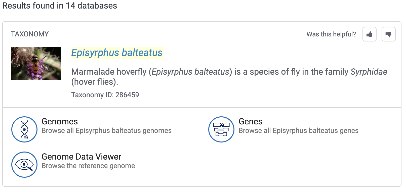
Generally, the first place to look reference genome data is at NCBI, https://ncbi.nlm.nih.gov, where you can start by simply typing the name of your organism in the search box at the home page — by means of example, let’s first search for the hoverfly Episyrphus balteatus:

For this species, we get the following “card” at the top of the results:

If you next click on “Genomes” in the result page above, you should get the following:

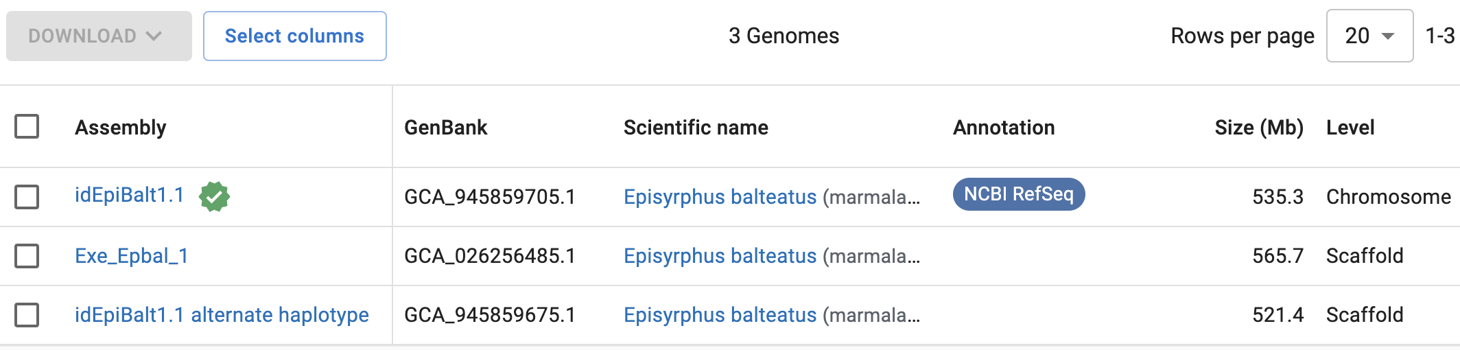
So, NCBI has 3 genomes assemblies for Episyrphus balteatus. The top one has a green check mark next to it (which means that this genome has been designated the primary reference genome for the focal organism), and it is also the only genome with an entry in the Annotation column and with a “Chromosome” (vs. “Scaffold”) assembly Level. Therefore, that top assembly, idEpiBalt1.1, would be the one to go with.

You can click on each assembly to get more information, including statistics like the number of scaffolds.

Your Turn: Now let’s switch to Culex. How many Culex assemblies are on NCBI (do a genus-wide search)? Are there any for Culex pipiens, and if so, which would you pick? (Click for the answer)

Go through the same process as shown above for Episyrphus balteatus, instead entering “Culex” in the search box.

You should find that there are 5 Culex assemblies, 2 of which are Culex pipiens. The first one, TS_CPP_V2, has the reference checkmark next to it and has an entry in the Annotation column, which the second one (TS_CPM_V1) doesn’t:

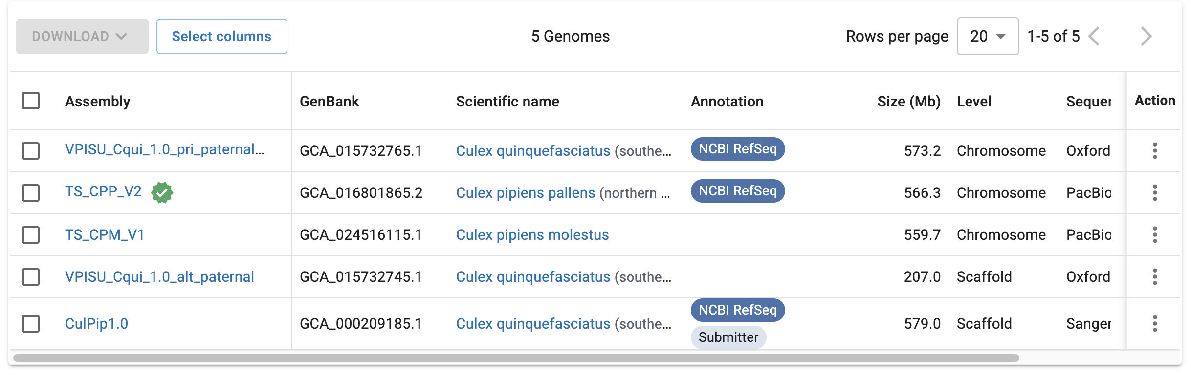
(These two are also from different subspecies, but as far as I could see, the authors of our study don’t specify the focal subspecies – though you could probably figure that out based on geographic range.)

As shown in the solutions above, there is currently a reference genome for Cx. pipiens available¹, and we’ll be “using” (looking at) that one. I have downloaded its files for you, which were among the files you just copied.

Your Turn: Take a closer look at our focal genome on the NCBI website. What is the size of the genome assembly? How many chromosomes and scaffolds does it contain? And how many protein-coding genes? (Click for the solutions)

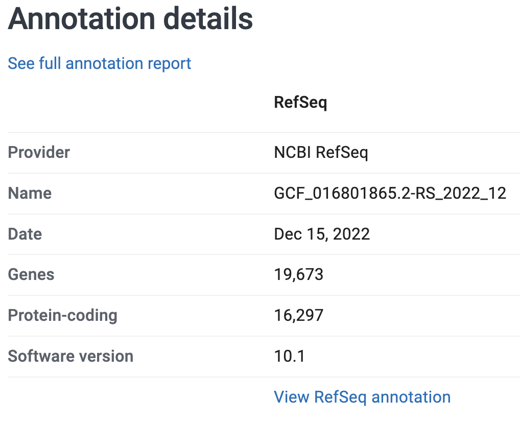
On the genome’s page at NCBI, some of the information includes the following stats on the assembly and the annotation:

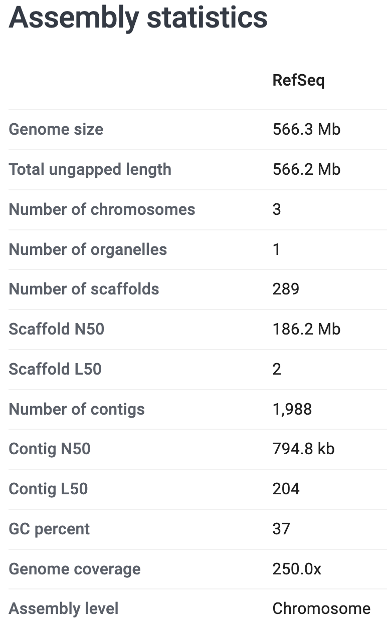
So:

It is 566.3 Mb (Megabases)
It contains 3 chromosomes and 289 unplaced scaffolds
It has 16,297 protein-coding genes

Side note: Downloading the reference genome files (Click to expand)

If you wanted to download the reference genome files from the NCBI website, you could either select an assembly in the overview table and click the Download button, or click the Download button at the top of the page for a specific assembly. That should get you the following pop-up window:

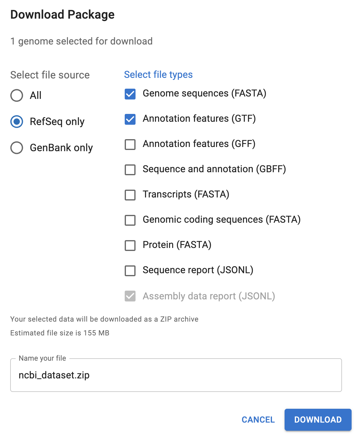
You’ll want to select at least the “Genome sequences (FASTA)” and one or both of the “Annotation features” files (GTF is often preferred with RNA-seq).

This allows you to download the data to your computer, and you could then upload it OSC. (Though a faster and more reproducible solution would be to use a command in your OSC shell to directly download these — the datasets and curl buttons next to the Download one a genome’s page help with that.)

Finally, if a “RefSeq” assembly is available, like it is for this genome, you’ll want to select that, as it has been curated and standardized by NCBI (whereas “GenBank” entries are exactly as submitted by researchers). This mostly makes a difference for the annotation rather than the assembly itself.

Side note: Reference genome complications (Click to expand)

Other useful database for reference genomes are Ensembl and the specialized databases that exist for certain organisms, like FlyBase for Drosophila, VectorBase mostly for mosquitos, and JGI Phytozome for plants.

In many cases, these databases don’t contain the exact same reference genome files than NCBI. Often, at least the annotation is different (and actually the product of an independent annotation effort), but even the assembly may have small differences including in chromosome/scaffold names, which can make these files completely incompatible. And to make matters even more complicated, it is not always clear which database is the best source for your genome.

Interestingly, the paper with the Cx. pipiens reference genome that we just found was already published in 2021, well before our focal Molecular Ecology paper.

And when we take a closer look at the quote from the paper, they say no genome for Cx. pipiens is “available in Ensembl” — which is in fact still the case. Could it be that the authors preferred the Ensembl genome from Cx. quinquefasciatus over the NCBI genome of Cx. pipiens? Or perhaps they just did their analyses already several years ago?

2.2 Reference genome files I: FASTA

The FASTA format

FASTA files contain one or more DNA or amino acid sequences, with no limits on the number of sequences or the sequence lengths. FASTA is the standard format for, e.g.:

Genome assembly sequences
Transcriptomes and proteomes (all of an organism’s transcripts & amino acid sequences, respectively)
Sequence downloads from NCBI such as a single gene/protein or other GenBank entry

The following example FASTA file contains two entries:

>unique_sequence_ID Optional description
ATTCATTAAAGCAGTTTATTGGCTTAATGTACATCAGTGAAATCATAAATGCTAAAAA
>unique_sequence_ID2
ATTCATTAAAGCAGTTTATTGGCTTAATGTACATCAGTGAAATCATAAATGCTAAATG

Each entry consists of a header line and the sequence itself. Header lines start with a > (greater-than sign) and are otherwise “free form”, though the idea is that they provide an identifier for the sequence that follows.²

FASTA file name extensions are variable: .fa, .fasta, .fna, .faa (Click to expand)

“Generic” extensions are .fasta and .fa (e.g: culex_assembly.fasta)
Also used are extensions that explicitly indicate whether sequences are nucleotides (.fna) or amino acids (.faa)

Your Culex genome assembly FASTA

Your reference genome files are in data/ref:

ls -lh data/ref

-rw------- 1 jelmer PAS0471 547M Jan 22 12:34 GCF_016801865.2.fna
-rw------- 1 jelmer PAS0471 123M Jan 22 12:34 GCF_016801865.2.gtf

While we can easily open small to medium-size files in the editor pane, “visual editors” like that do not work well for larger files like these.

A handy command to view text files of any size is less, which opens them up in a “pager” within your shell – you’ll see what that means if you try it with one of the assembly FASTA file:

less data/ref/GCF_016801865.2.fna

>NC_068937.1 Culex pipiens pallens isolate TS chromosome 1, TS_CPP_V2, whole genome shotgun sequence
aagcccttttatggtcaaaaatatcgtttaacttgaatatttttccttaaaaaataaataaatttaagcaaacagctgag
tagatgtcatctactcaaatctacccataagcacacccctgttcaatttttttttcagccataagggcgcctccagtcaa
attttcatattgagaatttcaatacaattttttaagtcgtaggggcgcctccagtcaaattttcatattgagaatttcaa
tacatttttttatgtcgtaggggcgcctccagtcaaattttcatattgagaatttcaatacattttttttaagtcgtagg
ggcgcctccagtcaaattttcatattgagaatttcaatacatttttttaagtcttaggggcgcctccagtcaaattttca
tattgagaatttcaatacatttttttaagtcgtaggggcgcctccagtcaaattttcatattgagaattttaatacaatt
ttttaaatcctaggggcgccttcagacaaacttaatttaaaaaatatcgctcctcgacttggcgactttgcgactgactg
cgacagcactaccttggaacactgaaatgtttggttgactttccagaaagagtgcatatgacttgaaaaaaaaagagcgc
ttcaaaattgagtcaagaaattggtgaaacttggtgcaagcccttttatggttaaaaatatcgtttaacttgaatatttt
tccttaaaaaataaataaatttaagcaaacagctgagtagatgtcatctactcaaatctacccataagcacacccctgga
CCTAATTCATGGAGGTGAATAGAGCATACGTAAATACAAAACTCATGACATTAGCCTGTAAGGATTGTGTaattaatgca
aaaatattgaTAGAATGAAAGATGCAAGTCccaaaaattttaagtaaatgaATAGTAATCATAAAGATAActgatgatga

Your Turn: Explore the file with less (Click to see the instructions)

After running the command above, the file should have “opened” inside the less pager.

You can move around in the file in several ways: by scrolling with your mouse, with up and down arrows, or, if you have them, PgUp and PgDn keys (also, u will move up half a page and d will move down half a page).

If you find yourself scrolling down and down to try and reach the end of the file, you can instead press G to go to the very end right away (and g to go back to the top).

Notice that you are “inside” this pager and won’t have your shell prompt back until you press q to quit less.

Side note: Lowercase vs. uppercase nucleotide letters? (Click to expand)

As you have probably noticed, nucleotide bases are typically typed in uppercase (A, C, G, T). What does the mixture of lowercase and uppercase bases in the Cx. pipiens assembly FASTA mean, then?

Lowercase bases are what is called “soft-masked”: they are repetitive sequences, and bioinformatics programs will treat them differently than non-repetitive sequences, which are in uppercase.

2.3 Reference genome files II: GFF/GTF

The GFF/GTF format

The GTF and GFF formats are very similar tab-delimited tabular files that contain genome annotations, with:

One row for each annotated “genomic feature” (gene, exon, etc.)
One column for each piece of information about a feature, like its genomic coordinates

See the sample below, with an added header line (not normally present) with column names:

seqname     source  feature start   end     score  strand  frame    attributes
NC_000001   RefSeq  gene    11874   14409   .       +       .       gene_id "DDX11L1"; transcript_id ""; db_xref "GeneID:100287102"; db_xref "HGNC:HGNC:37102"; description "DEAD/H-box helicase 11 like 1 (pseudogene)"; gbkey "Gene"; gene "DDX11L1"; gene_biotype "transcribed_pseudogene"; pseudo "true"; 
NC_000001   RefSeq  exon    11874   12227   .       +       .       gene_id "DDX11L1"; transcript_id "NR_046018.2"; db_xref "GeneID:100287102"; gene "DDX11L1"; product "DEAD/H-box helicase 11 like 1 (pseudogene)"; pseudo "true";

Some details on the more important/interesting columns:

seqname — Name of the chromosome, scaffold, or contig
feature — Name of the feature type, e.g. “gene”, “exon”, “intron”, “CDS”
start & end — Start & end position of the feature
strand — Whether the feature is on the + (forward) or - (reverse) strand
attribute — A semicolon-separated list of tag-value pairs with additional information

Your Culex GTF file

For our Cx. pipiens reference genome, we only have a GTF file.³
Take a look at it, again with less, but now with the -S option:

less -S data/ref/GCF_016801865.2.gtf

#gtf-version 2.2
#!genome-build TS_CPP_V2
#!genome-build-accession NCBI_Assembly:GCF_016801865.2
#!annotation-source NCBI RefSeq GCF_016801865.2-RS_2022_12
NC_068937.1     Gnomon  gene    2046    110808  .       +       .       gene_id "LOC120427725"; transcript_id ""; db_xref "GeneID:120427725"; description "homeotic protein deformed"; gbkey "Gene"; gene "LOC120427725"; gene_biotype "protein_coding"; 
NC_068937.1     Gnomon  transcript      2046    110808  .       +       .       gene_id "LOC120427725"; transcript_id "XM_052707445.1"; db_xref "GeneID:120427725"; gbkey "mRNA"; gene "LOC120427725"; model_evidence "Supporting evidence includes similarity to: 25 Proteins"; product "homeotic protein deformed, transcript variant X3"; transcript_biotype "mRNA"; 
NC_068937.1     Gnomon  exon    2046    2531    .       +       .       gene_id "LOC120427725"; transcript_id "XM_052707445.1"; db_xref "GeneID:120427725"; gene "LOC120427725"; model_evidence "Supporting evidence includes similarity to: 25 Proteins"; product "homeotic protein deformed, transcript variant X3"; transcript_biotype "mRNA"; exon_number "1"; 
NC_068937.1     Gnomon  exon    52113   52136   .       +       .       gene_id "LOC120427725"; transcript_id "XM_052707445.1"; db_xref "GeneID:120427725"; gene "LOC120427725"; model_evidence "Supporting evidence includes similarity to: 25 Proteins"; product "homeotic protein deformed, transcript variant X3"; transcript_biotype "mRNA"; exon_number "2"; 
NC_068937.1     Gnomon  exon    70113   70962   .       +       .       gene_id "LOC120427725"; transcript_id "XM_052707445.1"; db_xref "GeneID:120427725"; gene "LOC120427725"; model_evidence "Supporting evidence includes similarity to: 25 Proteins"; product "homeotic protein deformed, transcript variant X3"; transcript_biotype "mRNA"; exon_number "3"; 
NC_068937.1     Gnomon  exon    105987  106087  .       +       .       gene_id "LOC120427725"; transcript_id "XM_052707445.1"; db_xref "GeneID:120427725"; gene "LOC120427725"; model_evidence "Supporting evidence includes similarity to: 25 Proteins"; product "homeotic protein deformed, transcript variant X3"; transcript_biotype "mRNA"; exon_number "4"; 
NC_068937.1     Gnomon  exon    106551  106734  .       +       .       gene_id "LOC120427725"; transcript_id "XM_052707445.1"; db_xref "GeneID:120427725"; gene "LOC120427725"; model_evidence "Supporting evidence includes similarity to: 25 Proteins"; product "homeotic protein deformed, transcript variant X3"; transcript_biotype "mRNA"; exon_number "5";

Avoid line-wrapping with less -S

Lines in a file may contain too many characters to fit on your screen, as will be the case for this GTF file. less will by default “wrap” such lines onto the next line on your screen, but this is often confusing for files like FASTQ and tabular files like GTF. Therefore, we turned off line-wrapping above by using the -S option to less.

Your Turn: The GTF file is sorted: all entries from the first line of the table, until you again see “gene” in the third column, belong to the first gene. Can you make sense of all these entries for this gene, given what you know of gene structures? How many transcripts does this gene have? (Click to see some pointers)

The first gene (“LOC120427725”) has 3 transcripts.
Each transcript has 6-7 exons, 5 CDSs, and a start and stop codon.

Below, I’ve printed all lines belonging to the first gene:

NC_068937.1 Gnomon  gene    2046    110808  .   +   .   gene_id "LOC120427725"; transcript_id ""; db_xref "GeneID:120427725"; description "homeotic protein deformed"; gbkey "Gene"; gene "LOC120427725"; gene_biotype "protein_coding"; 
NC_068937.1 Gnomon  transcript  2046    110808  .   +   .   gene_id "LOC120427725"; transcript_id "XM_052707445.1"; db_xref "GeneID:120427725"; gbkey "mRNA"; gene "LOC120427725"; model_evidence "Supporting evidence includes similarity to: 25 Proteins"; product "homeotic protein deformed, transcript variant X3"; transcript_biotype "mRNA"; 
NC_068937.1 Gnomon  exon    2046    2531    .   +   .   gene_id "LOC120427725"; transcript_id "XM_052707445.1"; db_xref "GeneID:120427725"; gene "LOC120427725"; model_evidence "Supporting evidence includes similarity to: 25 Proteins"; product "homeotic protein deformed, transcript variant X3"; transcript_biotype "mRNA"; exon_number "1"; 
NC_068937.1 Gnomon  exon    52113   52136   .   +   .   gene_id "LOC120427725"; transcript_id "XM_052707445.1"; db_xref "GeneID:120427725"; gene "LOC120427725"; model_evidence "Supporting evidence includes similarity to: 25 Proteins"; product "homeotic protein deformed, transcript variant X3"; transcript_biotype "mRNA"; exon_number "2"; 
NC_068937.1 Gnomon  exon    70113   70962   .   +   .   gene_id "LOC120427725"; transcript_id "XM_052707445.1"; db_xref "GeneID:120427725"; gene "LOC120427725"; model_evidence "Supporting evidence includes similarity to: 25 Proteins"; product "homeotic protein deformed, transcript variant X3"; transcript_biotype "mRNA"; exon_number "3"; 
NC_068937.1 Gnomon  exon    105987  106087  .   +   .   gene_id "LOC120427725"; transcript_id "XM_052707445.1"; db_xref "GeneID:120427725"; gene "LOC120427725"; model_evidence "Supporting evidence includes similarity to: 25 Proteins"; product "homeotic protein deformed, transcript variant X3"; transcript_biotype "mRNA"; exon_number "4"; 
NC_068937.1 Gnomon  exon    106551  106734  .   +   .   gene_id "LOC120427725"; transcript_id "XM_052707445.1"; db_xref "GeneID:120427725"; gene "LOC120427725"; model_evidence "Supporting evidence includes similarity to: 25 Proteins"; product "homeotic protein deformed, transcript variant X3"; transcript_biotype "mRNA"; exon_number "5"; 
NC_068937.1 Gnomon  exon    109296  109660  .   +   .   gene_id "LOC120427725"; transcript_id "XM_052707445.1"; db_xref "GeneID:120427725"; gene "LOC120427725"; model_evidence "Supporting evidence includes similarity to: 25 Proteins"; product "homeotic protein deformed, transcript variant X3"; transcript_biotype "mRNA"; exon_number "6"; 
NC_068937.1 Gnomon  exon    109726  110808  .   +   .   gene_id "LOC120427725"; transcript_id "XM_052707445.1"; db_xref "GeneID:120427725"; gene "LOC120427725"; model_evidence "Supporting evidence includes similarity to: 25 Proteins"; product "homeotic protein deformed, transcript variant X3"; transcript_biotype "mRNA"; exon_number "7"; 
NC_068937.1 Gnomon  CDS 70143   70962   .   +   0   gene_id "LOC120427725"; transcript_id "XM_052707445.1"; db_xref "GeneID:120427725"; gbkey "CDS"; gene "LOC120427725"; product "homeotic protein deformed"; protein_id "XP_052563405.1"; exon_number "3"; 
NC_068937.1 Gnomon  CDS 105987  106087  .   +   2   gene_id "LOC120427725"; transcript_id "XM_052707445.1"; db_xref "GeneID:120427725"; gbkey "CDS"; gene "LOC120427725"; product "homeotic protein deformed"; protein_id "XP_052563405.1"; exon_number "4"; 
NC_068937.1 Gnomon  CDS 106551  106734  .   +   0   gene_id "LOC120427725"; transcript_id "XM_052707445.1"; db_xref "GeneID:120427725"; gbkey "CDS"; gene "LOC120427725"; product "homeotic protein deformed"; protein_id "XP_052563405.1"; exon_number "5"; 
NC_068937.1 Gnomon  CDS 109296  109660  .   +   2   gene_id "LOC120427725"; transcript_id "XM_052707445.1"; db_xref "GeneID:120427725"; gbkey "CDS"; gene "LOC120427725"; product "homeotic protein deformed"; protein_id "XP_052563405.1"; exon_number "6"; 
NC_068937.1 Gnomon  CDS 109726  110025  .   +   0   gene_id "LOC120427725"; transcript_id "XM_052707445.1"; db_xref "GeneID:120427725"; gbkey "CDS"; gene "LOC120427725"; product "homeotic protein deformed"; protein_id "XP_052563405.1"; exon_number "7"; 
NC_068937.1 Gnomon  start_codon 70143   70145   .   +   0   gene_id "LOC120427725"; transcript_id "XM_052707445.1"; db_xref "GeneID:120427725"; gbkey "CDS"; gene "LOC120427725"; product "homeotic protein deformed"; protein_id "XP_052563405.1"; exon_number "3"; 
NC_068937.1 Gnomon  stop_codon  110026  110028  .   +   0   gene_id "LOC120427725"; transcript_id "XM_052707445.1"; db_xref "GeneID:120427725"; gbkey "CDS"; gene "LOC120427725"; product "homeotic protein deformed"; protein_id "XP_052563405.1"; exon_number "7"; 
NC_068937.1 Gnomon  transcript  5979    110808  .   +   .   gene_id "LOC120427725"; transcript_id "XM_039592629.2"; db_xref "GeneID:120427725"; gbkey "mRNA"; gene "LOC120427725"; model_evidence "Supporting evidence includes similarity to: 24 Proteins"; product "homeotic protein deformed, transcript variant X2"; transcript_biotype "mRNA"; 
NC_068937.1 Gnomon  exon    5979    6083    .   +   .   gene_id "LOC120427725"; transcript_id "XM_039592629.2"; db_xref "GeneID:120427725"; gene "LOC120427725"; model_evidence "Supporting evidence includes similarity to: 24 Proteins"; product "homeotic protein deformed, transcript variant X2"; transcript_biotype "mRNA"; exon_number "1"; 
NC_068937.1 Gnomon  exon    52113   52136   .   +   .   gene_id "LOC120427725"; transcript_id "XM_039592629.2"; db_xref "GeneID:120427725"; gene "LOC120427725"; model_evidence "Supporting evidence includes similarity to: 24 Proteins"; product "homeotic protein deformed, transcript variant X2"; transcript_biotype "mRNA"; exon_number "2"; 
NC_068937.1 Gnomon  exon    70113   70962   .   +   .   gene_id "LOC120427725"; transcript_id "XM_039592629.2"; db_xref "GeneID:120427725"; gene "LOC120427725"; model_evidence "Supporting evidence includes similarity to: 24 Proteins"; product "homeotic protein deformed, transcript variant X2"; transcript_biotype "mRNA"; exon_number "3"; 
NC_068937.1 Gnomon  exon    105987  106087  .   +   .   gene_id "LOC120427725"; transcript_id "XM_039592629.2"; db_xref "GeneID:120427725"; gene "LOC120427725"; model_evidence "Supporting evidence includes similarity to: 24 Proteins"; product "homeotic protein deformed, transcript variant X2"; transcript_biotype "mRNA"; exon_number "4"; 
NC_068937.1 Gnomon  exon    106551  106734  .   +   .   gene_id "LOC120427725"; transcript_id "XM_039592629.2"; db_xref "GeneID:120427725"; gene "LOC120427725"; model_evidence "Supporting evidence includes similarity to: 24 Proteins"; product "homeotic protein deformed, transcript variant X2"; transcript_biotype "mRNA"; exon_number "5"; 
NC_068937.1 Gnomon  exon    109296  109660  .   +   .   gene_id "LOC120427725"; transcript_id "XM_039592629.2"; db_xref "GeneID:120427725"; gene "LOC120427725"; model_evidence "Supporting evidence includes similarity to: 24 Proteins"; product "homeotic protein deformed, transcript variant X2"; transcript_biotype "mRNA"; exon_number "6"; 
NC_068937.1 Gnomon  exon    109726  110808  .   +   .   gene_id "LOC120427725"; transcript_id "XM_039592629.2"; db_xref "GeneID:120427725"; gene "LOC120427725"; model_evidence "Supporting evidence includes similarity to: 24 Proteins"; product "homeotic protein deformed, transcript variant X2"; transcript_biotype "mRNA"; exon_number "7"; 
NC_068937.1 Gnomon  CDS 70143   70962   .   +   0   gene_id "LOC120427725"; transcript_id "XM_039592629.2"; db_xref "GeneID:120427725"; gbkey "CDS"; gene "LOC120427725"; product "homeotic protein deformed"; protein_id "XP_039448563.1"; exon_number "3"; 
NC_068937.1 Gnomon  CDS 105987  106087  .   +   2   gene_id "LOC120427725"; transcript_id "XM_039592629.2"; db_xref "GeneID:120427725"; gbkey "CDS"; gene "LOC120427725"; product "homeotic protein deformed"; protein_id "XP_039448563.1"; exon_number "4"; 
NC_068937.1 Gnomon  CDS 106551  106734  .   +   0   gene_id "LOC120427725"; transcript_id "XM_039592629.2"; db_xref "GeneID:120427725"; gbkey "CDS"; gene "LOC120427725"; product "homeotic protein deformed"; protein_id "XP_039448563.1"; exon_number "5"; 
NC_068937.1 Gnomon  CDS 109296  109660  .   +   2   gene_id "LOC120427725"; transcript_id "XM_039592629.2"; db_xref "GeneID:120427725"; gbkey "CDS"; gene "LOC120427725"; product "homeotic protein deformed"; protein_id "XP_039448563.1"; exon_number "6"; 
NC_068937.1 Gnomon  CDS 109726  110025  .   +   0   gene_id "LOC120427725"; transcript_id "XM_039592629.2"; db_xref "GeneID:120427725"; gbkey "CDS"; gene "LOC120427725"; product "homeotic protein deformed"; protein_id "XP_039448563.1"; exon_number "7"; 
NC_068937.1 Gnomon  start_codon 70143   70145   .   +   0   gene_id "LOC120427725"; transcript_id "XM_039592629.2"; db_xref "GeneID:120427725"; gbkey "CDS"; gene "LOC120427725"; product "homeotic protein deformed"; protein_id "XP_039448563.1"; exon_number "3"; 
NC_068937.1 Gnomon  stop_codon  110026  110028  .   +   0   gene_id "LOC120427725"; transcript_id "XM_039592629.2"; db_xref "GeneID:120427725"; gbkey "CDS"; gene "LOC120427725"; product "homeotic protein deformed"; protein_id "XP_039448563.1"; exon_number "7"; 
NC_068937.1 Gnomon  transcript  60854   110807  .   +   .   gene_id "LOC120427725"; transcript_id "XM_039592628.2"; db_xref "GeneID:120427725"; gbkey "mRNA"; gene "LOC120427725"; model_evidence "Supporting evidence includes similarity to: 24 Proteins"; product "homeotic protein deformed, transcript variant X1"; transcript_biotype "mRNA"; 
NC_068937.1 Gnomon  exon    60854   61525   .   +   .   gene_id "LOC120427725"; transcript_id "XM_039592628.2"; db_xref "GeneID:120427725"; gene "LOC120427725"; model_evidence "Supporting evidence includes similarity to: 24 Proteins"; product "homeotic protein deformed, transcript variant X1"; transcript_biotype "mRNA"; exon_number "1"; 
NC_068937.1 Gnomon  exon    70113   70962   .   +   .   gene_id "LOC120427725"; transcript_id "XM_039592628.2"; db_xref "GeneID:120427725"; gene "LOC120427725"; model_evidence "Supporting evidence includes similarity to: 24 Proteins"; product "homeotic protein deformed, transcript variant X1"; transcript_biotype "mRNA"; exon_number "2"; 
NC_068937.1 Gnomon  exon    105987  106087  .   +   .   gene_id "LOC120427725"; transcript_id "XM_039592628.2"; db_xref "GeneID:120427725"; gene "LOC120427725"; model_evidence "Supporting evidence includes similarity to: 24 Proteins"; product "homeotic protein deformed, transcript variant X1"; transcript_biotype "mRNA"; exon_number "3"; 
NC_068937.1 Gnomon  exon    106551  106734  .   +   .   gene_id "LOC120427725"; transcript_id "XM_039592628.2"; db_xref "GeneID:120427725"; gene "LOC120427725"; model_evidence "Supporting evidence includes similarity to: 24 Proteins"; product "homeotic protein deformed, transcript variant X1"; transcript_biotype "mRNA"; exon_number "4"; 
NC_068937.1 Gnomon  exon    109296  109660  .   +   .   gene_id "LOC120427725"; transcript_id "XM_039592628.2"; db_xref "GeneID:120427725"; gene "LOC120427725"; model_evidence "Supporting evidence includes similarity to: 24 Proteins"; product "homeotic protein deformed, transcript variant X1"; transcript_biotype "mRNA"; exon_number "5"; 
NC_068937.1 Gnomon  exon    109726  110807  .   +   .   gene_id "LOC120427725"; transcript_id "XM_039592628.2"; db_xref "GeneID:120427725"; gene "LOC120427725"; model_evidence "Supporting evidence includes similarity to: 24 Proteins"; product "homeotic protein deformed, transcript variant X1"; transcript_biotype "mRNA"; exon_number "6"; 
NC_068937.1 Gnomon  CDS 70143   70962   .   +   0   gene_id "LOC120427725"; transcript_id "XM_039592628.2"; db_xref "GeneID:120427725"; gbkey "CDS"; gene "LOC120427725"; product "homeotic protein deformed"; protein_id "XP_039448562.1"; exon_number "2"; 
NC_068937.1 Gnomon  CDS 105987  106087  .   +   2   gene_id "LOC120427725"; transcript_id "XM_039592628.2"; db_xref "GeneID:120427725"; gbkey "CDS"; gene "LOC120427725"; product "homeotic protein deformed"; protein_id "XP_039448562.1"; exon_number "3"; 
NC_068937.1 Gnomon  CDS 106551  106734  .   +   0   gene_id "LOC120427725"; transcript_id "XM_039592628.2"; db_xref "GeneID:120427725"; gbkey "CDS"; gene "LOC120427725"; product "homeotic protein deformed"; protein_id "XP_039448562.1"; exon_number "4"; 
NC_068937.1 Gnomon  CDS 109296  109660  .   +   2   gene_id "LOC120427725"; transcript_id "XM_039592628.2"; db_xref "GeneID:120427725"; gbkey "CDS"; gene "LOC120427725"; product "homeotic protein deformed"; protein_id "XP_039448562.1"; exon_number "5"; 
NC_068937.1 Gnomon  CDS 109726  110025  .   +   0   gene_id "LOC120427725"; transcript_id "XM_039592628.2"; db_xref "GeneID:120427725"; gbkey "CDS"; gene "LOC120427725"; product "homeotic protein deformed"; protein_id "XP_039448562.1"; exon_number "6"; 
NC_068937.1 Gnomon  start_codon 70143   70145   .   +   0   gene_id "LOC120427725"; transcript_id "XM_039592628.2"; db_xref "GeneID:120427725"; gbkey "CDS"; gene "LOC120427725"; product "homeotic protein deformed"; protein_id "XP_039448562.1"; exon_number "2"; 
NC_068937.1 Gnomon  stop_codon  110026  110028  .   +   0   gene_id "LOC120427725"; transcript_id "XM_039592628.2"; db_xref "GeneID:120427725"; gbkey "CDS"; gene "LOC120427725"; product "homeotic protein deformed"; protein_id "XP_039448562.1"; exon_number "6";

3 FASTQ files

3.1 The FASTQ format

FASTQ is the standard HTS read data file format. Like the other genomic data files we’ve seen so far, these are plain text files. Each read forms one FASTQ entry and is represented by four lines:

A header that starts with @ and e.g. uniquely identifies the read
The sequence itself
A + (plus sign — yes, that’s all!)
One-character quality scores for each base in the sequence

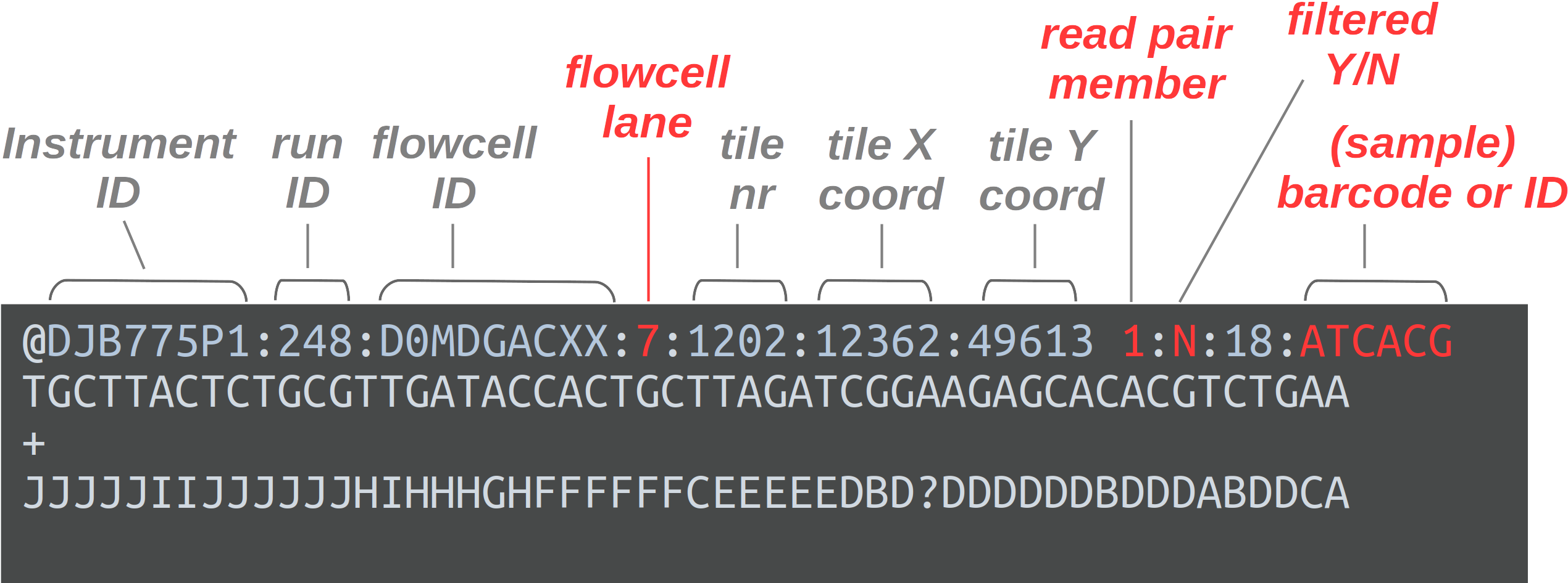
One entry (read) in a FASTQ file covers 4 lines.
The header line is annotated, with some of the more useful components highlighted in red.
For viewing purposes, this read (at only 56 bp) is shorter than what is typical.

Side note: FASTQ quality scores (Click to expand)

The quality scores we saw in the read above represent an estimate of the error probability of the base call.

Specifically, they correspond to a numeric “Phred” quality score (Q), which is a function of the estimated probability that a base call is erroneous (P):

Q = -10 * log10(P)

For some specific probabilities and their rough qualitative interpretation for Illumina data:

Phred quality score	Error probability	Rough interpretation
10	1 in 10	terrible
20	1 in 100	bad
30	1 in 1,000	good
40	1 in 10,000	excellent

This numeric quality score is represented in FASTQ files not by the number itself, but by a corresponding “ASCII character”. This allows for a single-character representation of each possible score — as a consequence, each quality score character can conveniently correspond to (& line up with) a base character in the read.

Phred quality score	Error probability	ASCII character
10	1 in 10	`+`
20	1 in 100	`5`
30	1 in 1,000	`?`
40	1 in 10,000	`I`

In practice, you almost never have to manually check the quality scores of bases in FASTQ files, but if you do, a rule of thumb is that letter characters are good (Phred of 32 and up). For your reference, here is a complete lookup table (look at the top table (BASE=33)).

3.2 Listing your FASTQ files

First, let’s take another look at your list of FASTQ files:

ls -lh data/fastq

-rw-r--r-- 1 jelmer PAS0471 21M Jan 21 13:36 ERR10802863_R1.fastq.gz
-rw-r--r-- 1 jelmer PAS0471 22M Jan 21 13:36 ERR10802863_R2.fastq.gz
-rw-r--r-- 1 jelmer PAS0471 21M Jan 21 13:36 ERR10802864_R1.fastq.gz
-rw-r--r-- 1 jelmer PAS0471 22M Jan 21 13:36 ERR10802864_R2.fastq.gz
-rw-r--r-- 1 jelmer PAS0471 22M Jan 21 13:36 ERR10802865_R1.fastq.gz
-rw-r--r-- 1 jelmer PAS0471 22M Jan 21 13:36 ERR10802865_R2.fastq.gz
[...truncated...]

In the file listing above:

First, take note of the file sizes. They are “only” about 22 Mb in size, and all have a very similar size. This is because I “subsampled” the FASTQ files to only have 500,000 reads per file. The original files were on average over 1 Gb in size with about 30 million reads.
Second, if you look closely at the file names, it looks like we have two FASTQ files per sample: one with _R1 at the end of the file name, and one with _R2.

Your Turn: What might each of the two files per sample represent/contain? (Click for the solution)

These contain the forward reads (_R1.fastq.gz) vs. the reverse reads (_R2.fastq.gz).

Your Turn: Do you have any idea why the file extension ends in .gz? (Click for the solution)

This means it is gzip-compressed. This saves a lot of space: compressed files can be up to 10 times smaller than uncompressed files. Most bioinformatics tools, including FastQC which we’ll run in a bit, can work with gzipped files directly, so there is no need to unzip them.

3.3 Viewing your FASTQ files

Despite the gzip-compression, we can simply use the less command as before to view the FASTQ files (!):

less data/fastq/ERR10802863_R1.fastq.gz

@ERR10802863.8435456 8435456 length=74
CAACGAATACATCATGTTTGCGAAACTACTCCTCCTCGCCTTGGTGGGGATCAGTACTGCGTACCAGTATGAGT
+
AAAAAEEEEEEEEEEEEEEEEEEEEEEEEEEEEEEEEEEEEEEEEEEEEEEEEEEEEEEEEEEEEEEEEEEEEE
@ERR10802863.27637245 27637245 length=74
GCCACACTTTTGAAGAACAGCGTCATTGTTCTTAATTTTGTCGGCAACGCCTGCACGAGCCTTCCACGTAAGTT
+
AAAAAEEEEEEEEEEEEEEEEEEEEEEEEEEEEEEEEEAEE<EEEEEEEEEEEEEEEEEEEEEEEEEEEEEEEE

Different header lines

The header lines (starting with @) are quite different from the earlier example, because these files were downloaded from SRA. When you get files directly from a (Illumina) sequencer, they will have headers much like the earlier example.

In practice, we don’t often have to closely look at the contents of our FASTQ files ourselves. There are simply too many reads to make sense of!

Instead, we’ll have specialized tools like FastQC summarize them for us: e.g. how many sequences there are, what the quality scores look like, and if there are adapter sequences. We’ll run FastQC below.

Your Turn: All of that said, in this case, you should be able to spot some very different-looking reads soon when looking at the file with less. What are they? (Click for the solution)

The 5^th read looks as follows — and if you scroll down you should quickly see several more reads like this:

@ERR10802863.11918285 11918285 length=35
NNNNNNNNNNNNNNNNNNNNNNNNNNNNNNNNNNN
+
###################################

These only consists of N bases (and they are also shorter than the other reads), and are therefore completely useless!

FYI: It not common to run into these kinds of failed reads as easily!

4 Quality control with FastQC

A good example of a tool with a command-line interface is FastQC, for quality control of FASTQ files. FastQC is ubiquitous: nearly all HTS data comes in FASTQ files, and the first step is always to check the read quality.

4.1 Running FastQC

To run FastQC, use the command fastqc.

If you want to analyze one of your FASTQ files with default FastQC settings, a complete FastQC command to do so would simply be fastqc followed by the name of the file⁴:

# (Don't run this)
fastqc data/fastq/ERR10802863_R1.fastq.gz

However, an annoying default behavior by FastQC is that it writes its output files in the dir where the input files are — in general, it’s not great practice to directly mix your primary data and results like that!

To figure out how we can change that behavior, first consider that many commands and bioinformatics tools alike have an option -h and/or --help to print usage information to the screen.

Your Turn: Try to print FastQC’s help info, and figure out which option you can use to specify an output directory of your choice. (Click for the solution)

fastqc -h and fastqc --help will both work to show the help info.

You’ll get quite a bit of output printed to screen, including the snippet about output directories that is reproduced below:

fastqc -h

  -o --outdir     Create all output files in the specified output directory.
                    Please note that this directory must exist as the program
                    will not create it.  If this option is not set then the 
                    output file for each sequence file is created in the same
                    directory as the sequence file which was processed.

So, you can use -o or equivalently, --outdir to specify an output dir.

Now, let’s try to run FastQC and tell it to use the output dir results/fastqc:

fastqc --outdir results/fastqc data/fastq/ERR10802863_R1.fastq.gz

bash: fastqc: command not found...

However, there is a wrinkle, as you can see above. It turns out that FastQC is installed at OSC⁵, but we have to “load it” before we can use it. Without having time to go into further details about software usage at OSC, please accept that we can load FastQC as follows:

module load fastqc

Now, let’s try again:

fastqc --outdir results/fastqc data/fastq/ERR10802863_R1.fastq.gz

Specified output directory 'results/fastqc' does not exist

Your Turn: Now what is going on this time? (Or had you perhaps seen this coming given the help text we saw earlier?) Can you try to fix the problem? (Click here for hints)

You’ll need to create a new directory, which you can do either by using the buttons in the VS Code side bar, or with the mkdir command — here, try it as mkdir -p followed by the name (path) of the directory you want to create.

Exercise solution (Click to expand)

The problem, as the error fairly clearly indicates, is that the output directory that we specified with --outdir does not currently exist. We might have expected FastQC to be smart/flexible enough to create this dir for us (many bioinformatics tools are), but alas. On the other hand, if we had read the help text clearly, it did warn us about this.
With the mkdir command, to create “two levels” of dirs at once, like we need to here (both results and then fastqc within there), we need its -p option:

mkdir -p results/fastqc

And for our final try before we give up and throw our laptop out the window (make sure to run the code in the exercise solution before you retry!):

fastqc --outdir results/fastqc data/fastq/ERR10802863_R1.fastq.gz

Started analysis of ERR10802863_R1.fastq.gz
Approx 5% complete for ERR10802863_R1.fastq.gz
Approx 10% complete for ERR10802863_R1.fastq.gz
Approx 15% complete for ERR10802863_R1.fastq.gz
[...truncated...]
Analysis complete for ERR10802863_R1.fastq.gz

Success!! (That should have taken just a few seconds with our subsampled FASTQ files.)

4.2 FastQC output files

Let’s take a look at the files in the output dir we specified:

ls -lh results/fastqc

-rw-r--r-- 1 jelmer PAS0471 241K Jan 25 15:50 ERR10802863_R1_fastqc.html
-rw-r--r-- 1 jelmer PAS0471 256K Jan 25 15:50 ERR10802863_R1_fastqc.zip

There is a .zip file, which contains tables with FastQC’s data summaries
There is an .html (HTML) file, which contains plots — this is what we’ll look at next

Your Turn: Run FastQC for the corresponding R2 file. Would you use the same output dir? (Click for the solution)

Yes, it makes sense to use the same output dir, since as you could see above, the output file names have the input file identifiers in them. As such, we don’t need to worry about overwriting files, and it will be easier to have all the results in a single dir.

To run FastQC for the R2 (=reverse-read) file:

fastqc --outdir results/fastqc ERR10802863_R2.fastq.gz

Started analysis of ERR10802863_R2.fastq.gz
Approx 5% complete for ERR10802863_R2.fastq.gz
Approx 10% complete for ERR10802863_R2.fastq.gz
Approx 15% complete for ERR10802863_R2.fastq.gz
[...truncated...]
Analysis complete for ERR10802863_2.fastq.gz

ls -lh results/fastqc

-rw-r--r-- 1 jelmer PAS0471 241K Jan 21 21:50 ERR10802863_R1_fastqc.html
-rw-r--r-- 1 jelmer PAS0471 256K Jan 21 21:50 ERR10802863_R1_fastqc.zip
-rw-r--r-- 1 jelmer PAS0471 234K Jan 21 21:53 ERR10802863_R2_fastqc.html
-rw-r--r-- 1 jelmer PAS0471 244K Jan 21 21:53 ERR10802863_R2_fastqc.zip

Now, we have four files: two for each of our preceding successful FastQC runs.

4.3 Interpreting FastQC’s output

First, we’ll unfortunately have to download FastQC’s output HTML files⁶:

Find the FastQC HTML files in the file explorer in the VS Code side bar.
Right-click on one of them, click Download... and follow the prompt to download the file somewhere to your computer (doesn’t matter where, just make sure you see where it goes).
Repeat this for the second file
Then, open your computer’s file browser, find the downloaded files, and double-click on one. It should be opened in your default web browser.

We’ll now go through a couple of the FastQC plots/modules, with first some example plots with good/bad results for reference.

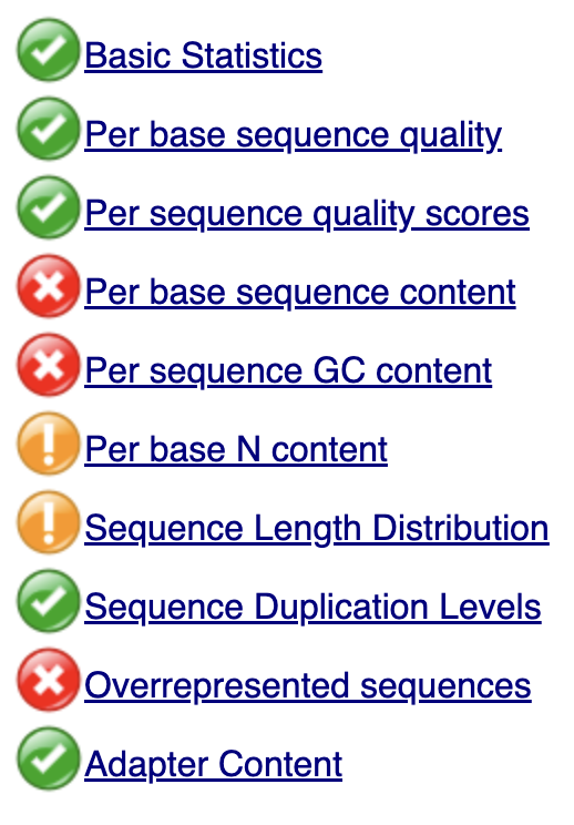
Overview of module results

FastQC has “pass” (checkmark in green), “warning” (exclamation mark in orange), and “fail” (cross in red) assessments for each module, as you can see below.

These are handy and typically at least somewhat meaningful, but it is important to realize that a “warning” or a “fail” is not necessarily the bad news that it may appear to be, because, e.g.:

Some of these modules could perhaps be called overly strict.
Some warnings and fails are easily remedied or simply not a very big deal.
FastQC assumes that your data is derived from whole-genome shotgun sequencing — some other types of data like RNA-seq data will always trigger a couple of warnings and files based on expected differences.

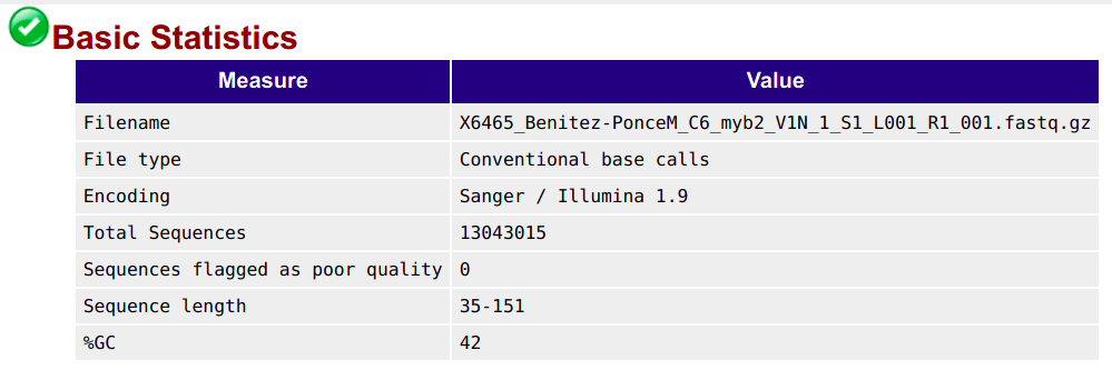
Basic statistics

This shows, for example, the number of sequences (reads) and the read length range for your file:

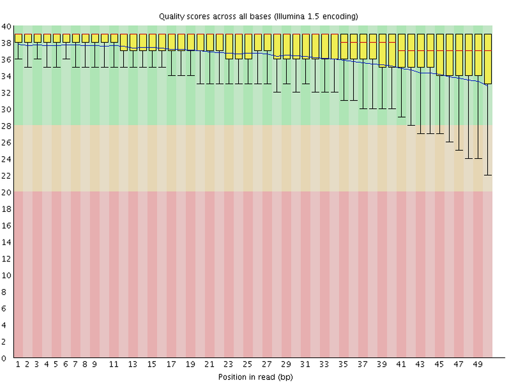
Per base quality sequence quality

This figure visualize the mean per-base quality score (y-axis) along the length of the reads (x-axis). Note that:

A decrease in sequence quality along the reads is normal.
R2 (reverse) reads are usually worse than R1 (forward) reads.

Good / acceptable:

Bad:

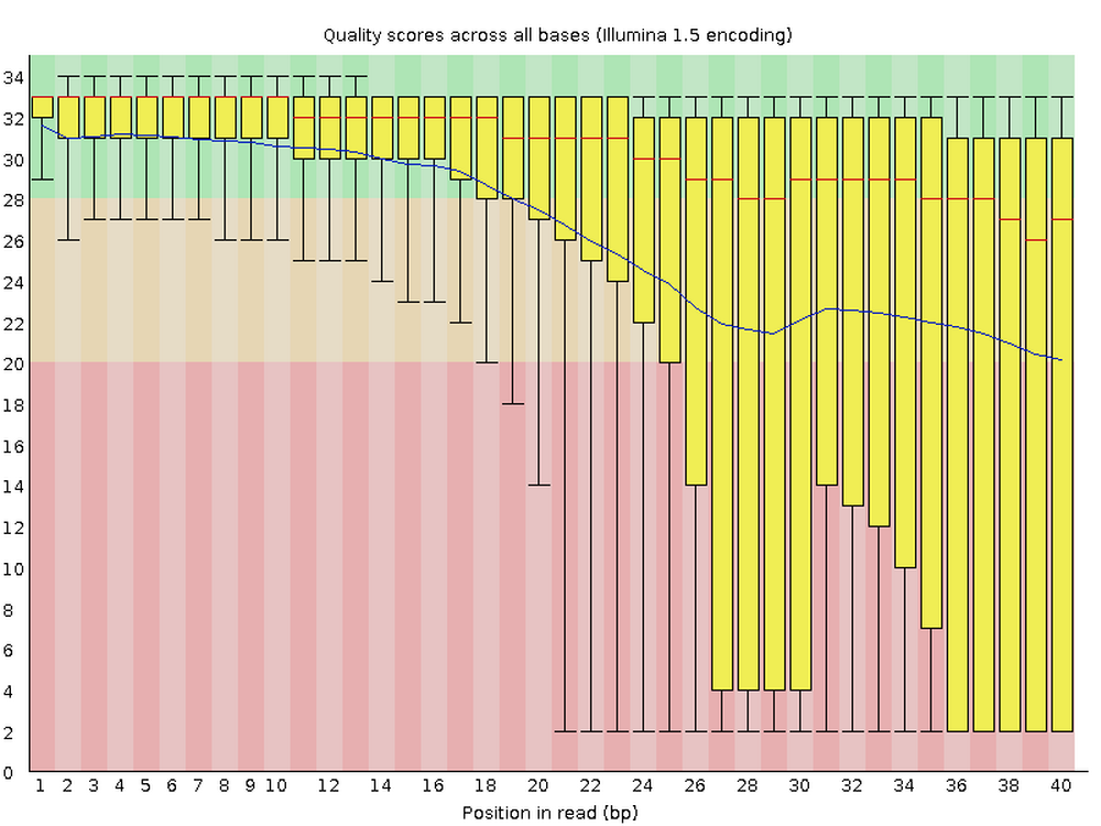
To interpret the quality scores along the y-axis, note the color scaling in the graphs (green is good, etc.), and see this table for details:

Phred quality score	Error probability	Rough interpretation
10	1 in 10	terrible
20	1 in 100	bad
30	1 in 1,000	good
40	1 in 10,000	excellent

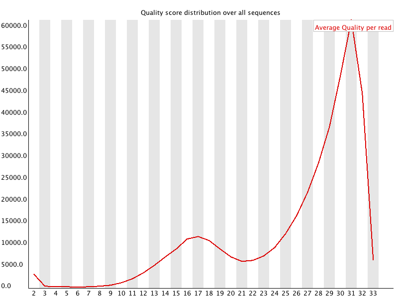
Per sequence quality scores

This shows the same quality scores we saw above, but now simply as a density plot of per-read averages, with the quality score now along the x-axis, and the number of reads with that quality score along the y-axis:

Good:

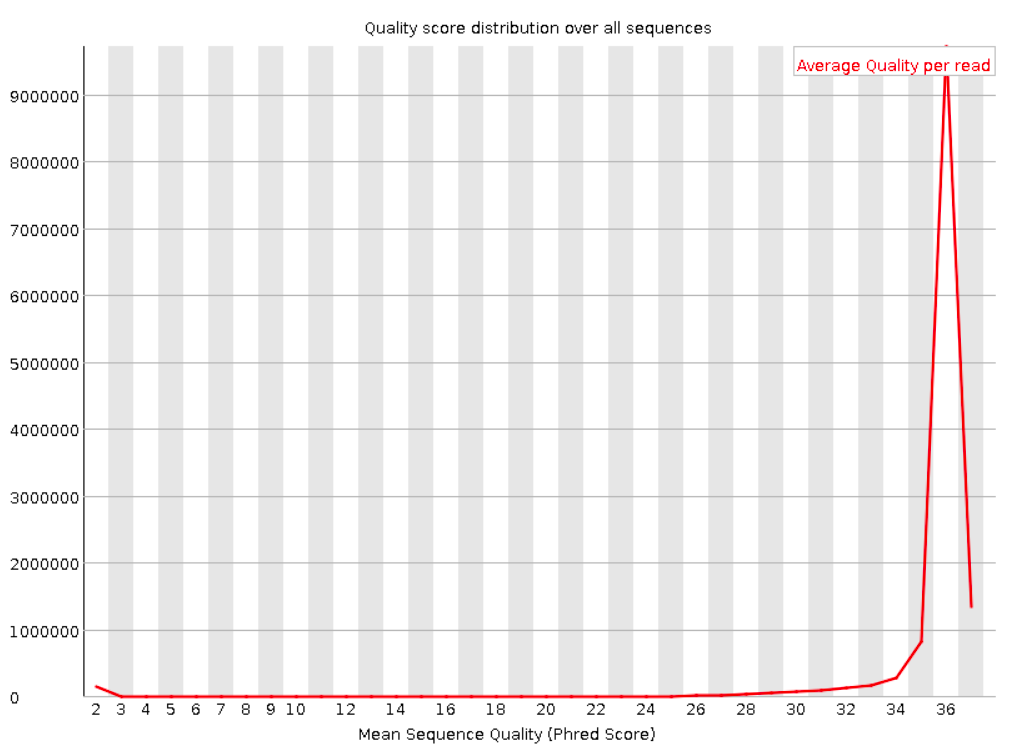
Bad:

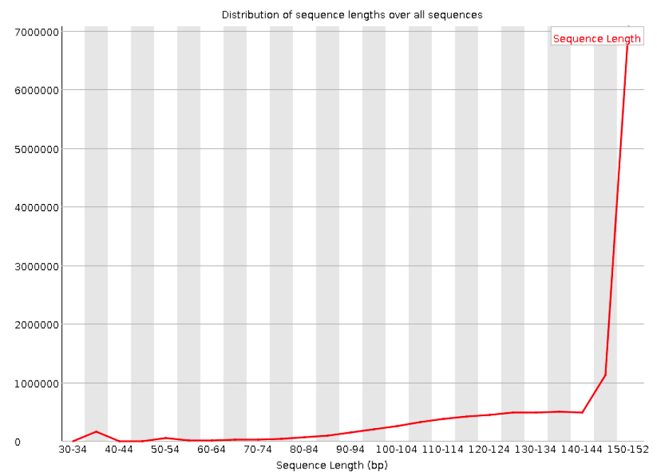
Sequence length distribution

Will throw a warning as soon as not all sequences are of the same length (like below), but this is quite normal.

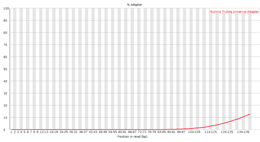
Adapter content

Checks for known adapter sequences. When some of the insert sizes are shorter than the read length, adapters can end up in the sequence – these should be removed!

Good:

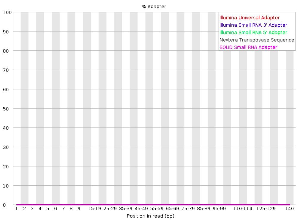
Bad:

4.4 Interpreting our FastQC output

Your Turn: Open the HTML file for the R1 FASTQ file and go through the modules we discussed above. Can you make sense of it? Does the data look good to you, overall?

Your Turn: Now open the HTML file for the R2 FASTQ file and take a look just at the quality scores. Does it look any worse than the R1?

5 In closing

In today’s lab, you were introduced to:

Working at the Ohio Supercomputer Center
Using the VS Code text editor
Using the Unix shell
Reference genome FASTA & GTF files & where to find these
HTS read FASTQ files and how to quality-control these
How to run a command-line bioinformatics tool

Taking a step back, I’ve shown you the main pieces of the computational infrastructure for what we may call “command-line genomics”: genomics analysis using command-line tools. And we’ve seen a basic example of loading and running a command-line tool at OSC.

Side note: scaling the analysis & next steps for real projects (Click to expand)

The missing pieces for a typical, fuller example of how such tools are run in the context of an actual genomics project are (if we stay with FastQC):

Putting the command to run FastQC in a “shell script”.
Submitting the script to the SLURM scheduler queue as a “batch job”.
To make speed things, using the OSC’s capabilities, we can submit multiple jobs in parallel using a loop.

If it seems that speed and computing power may not be an issue, given how fast FastQC ran, keep in mind that:

We here worked with subsampled (much smaller than usual) FASTQ files
We only ran FastQC for one of our 23 samples, and your experiment may have 50+ samples
We need to run a bunch more tools, and some of those take much longer to run or need lots of RAM memory.

All that said, those missing pieces mentioned above are outside the scope of this short introduction — but if you managed today, it should not be hard to learn those skills either.

6 Appendix

Bonus exercises

Your Turn (Bonus): Explore the assembly FASTA file with grep (Click to see the instructions)

grep is an incredibly useful Unix command with which you can search files for specific text. By default, it will print lines that match your search in their entirety.

For example, we could search the genome for the short sequence ACCGATACGACG:

grep "ACCGATACGACG" data/ref/GCF_016801865.2.fna

aaaatcgaaaaacgcgTTTACCTTACATTGACAAAGTTGACCGATACGACGGCTCGATGTGCCAAACCGGTCACAAAGTC
AATATTGACATTTCTTTTGCATTCTTCAGGTTCAGTGACCACAAACGGGACCGATACGACGGCTACCATCGGAATGCACC
TCAAAATGTGTCAATTAACGTAACTAGATTTTTACGATCATAATAAGTAGATACCGATACGACGGGGCGGCATTTATGCT
TAAGTAGATACCGATACGACGGGGCGGCATTCATGCTGCTACAGGGCTCAGCGGACCGACAAGCGACTGTGAAACGCAGC

(Matches should be highlighted in red, but that doesn’t show here, unfortunately)

Or count the number of times the much shorter sequence GGACC occurs:

grep -c "GGACC" data/ref/GCF_016801865.2.fna

Try to adapt the above example to:

Print all entry headers in the assembly FASTA file
Count the number of entry header (= the number of entries) in the assembly FASTA file

Does the number of entries make sense given how many chromosomes and scaffolds the assembly consists of according to NCBI?

Bonus exercise solutions (Click to expand)

To print all FASTA entry headers, simply search for > with grep (since > should not occur in the sequences themselves, which can only be bases or N). Make sure to uses quotes (">")!

grep ">" data/ref/GCF_016801865.2.fna

>NC_068937.1 Culex pipiens pallens isolate TS chromosome 1, TS_CPP_V2, whole genome shotgun sequence
>NC_068938.1 Culex pipiens pallens isolate TS chromosome 2, TS_CPP_V2, whole genome shotgun sequence
>NC_068939.1 Culex pipiens pallens isolate TS chromosome 3, TS_CPP_V2, whole genome shotgun sequence
>NW_026292818.1 Culex pipiens pallens isolate TS unplaced genomic scaffold, TS_CPP_V2 Cpp_Un0001, whole genome shotgun sequence
>NW_026292819.1 Culex pipiens pallens isolate TS unplaced genomic scaffold, TS_CPP_V2 Cpp_Un0002, whole genome shotgun sequence
>NW_026292820.1 Culex pipiens pallens isolate TS unplaced genomic scaffold, TS_CPP_V2 Cpp_Un0003, whole genome shotgun sequence
>NW_026292821.1 Culex pipiens pallens isolate TS unplaced genomic scaffold, TS_CPP_V2 Cpp_Un0004, whole genome shotgun sequence
[...truncated...]

We can count the number of header lines by modifying our above command only with the addition of the -c option:

grep -c ">" data/ref/GCF_016801865.2.fna

Attribution

Some of the FastQC example plots were taken from here.

Footnotes

But see the box below for more info/context↩︎
Note that because individual sequence entries are commonly spread across multiple lines, FASTA entries do not necessarily cover 2 lines (cf. FASTQ).↩︎
A GFF file would contain the same information but in a slightly different format. For programs used in RNA-seq analysis, GTF files tend to be the preferred format.↩︎
Note that this is very similar to running, say, the ls command!↩︎
For a full list of installed software at OSC: https://www.osc.edu/resources/available_software/software_list ↩︎
The installed version of VS Code does not allow us to view HTML files↩︎