Introduction to R and RStudio

Week 11 – lecture A

Authors

Affiliation

Menuka Bhandari

CFAES Bioinformatics Core, Ohio State University

Jelmer Poelstra

Published

November 1, 2025

1 Introduction

1.1 Overview and learning goals of the course’s R material

This is the first of four-weeks series that will focus on the R language. Besides being a great all-round tool for data analysis and visualization, the R language is probably the best environment for the “downstream” analysis of omics data, with an excellent array of packages for e.g.:

Metabarcoding analysis
RNA-Seq analysis
Lipidomics
Proteomics and metabolomics

Specifically, you will learn:

The basics of R (this lecture)
How data is stored in R, using e.g. vectors and different data types (next lecture)
How to use Quarto to produce beautiful, reproducible documents (week 12)
How to visualize data in R with the ggplot2 package (week 13)
About the ecosystem of packages for omics data analysis (week 13/14)
By means of example, how to analyze the RNA-Seq count data you have produced using the Garrigós et al. (2025) dataset.

1.2 Lecture learning goals

In this lecture, you will learn:

The RStudio layout and the functions of the different panes and tabs
The basics of interacting with R by using R as a calculator
Defining a variables/objects in R, and assigning values/data to them
Calling R functions
Installing and loading R packages
Getting help in R

2 Starting an RStudio Server session at OSC

You can use R with a “console” that can simply be run inside the terminal (at OSC, you can do so after loading the R module). However, we’ll use R with a fancy editor (or “IDE”, Integrated Development Environment) called RStudio, which makes working with it much more pleasant!

Similar to VS Code, we can run a version of RStudio (“RStudio Server”) within our browsers by starting an Interactive App through OSC OnDemand.

Log in to OSC’s OnDemand portal at https://ondemand.osc.edu
In the blue top bar, select Interactive Apps at the bottom, click RStudio Server
Fill out the form as follows:
- Cluster: pitzer
- R version: 4.4.0
- Project: PAS2880
- Number of hours: 2
- Node type: any
- Number of cores: 1
Click Launch
Click the Connect to RStudio Server button once it appears

Number of cores

Note that unlike with Code Server, we can choose how many cores we want when starting an RStudio server job. Changing the number of cores is also the way to go if you need more than the default 4 GB of memory (RAM): recall that each core is associated with 4 GB of memory, so asking for 4 cores will get you 16 GB RAM.

Installing R on your own computer

While you don’t need to do so for this course, you can also easily install R and RStudio on your computer. For more information, see this page.

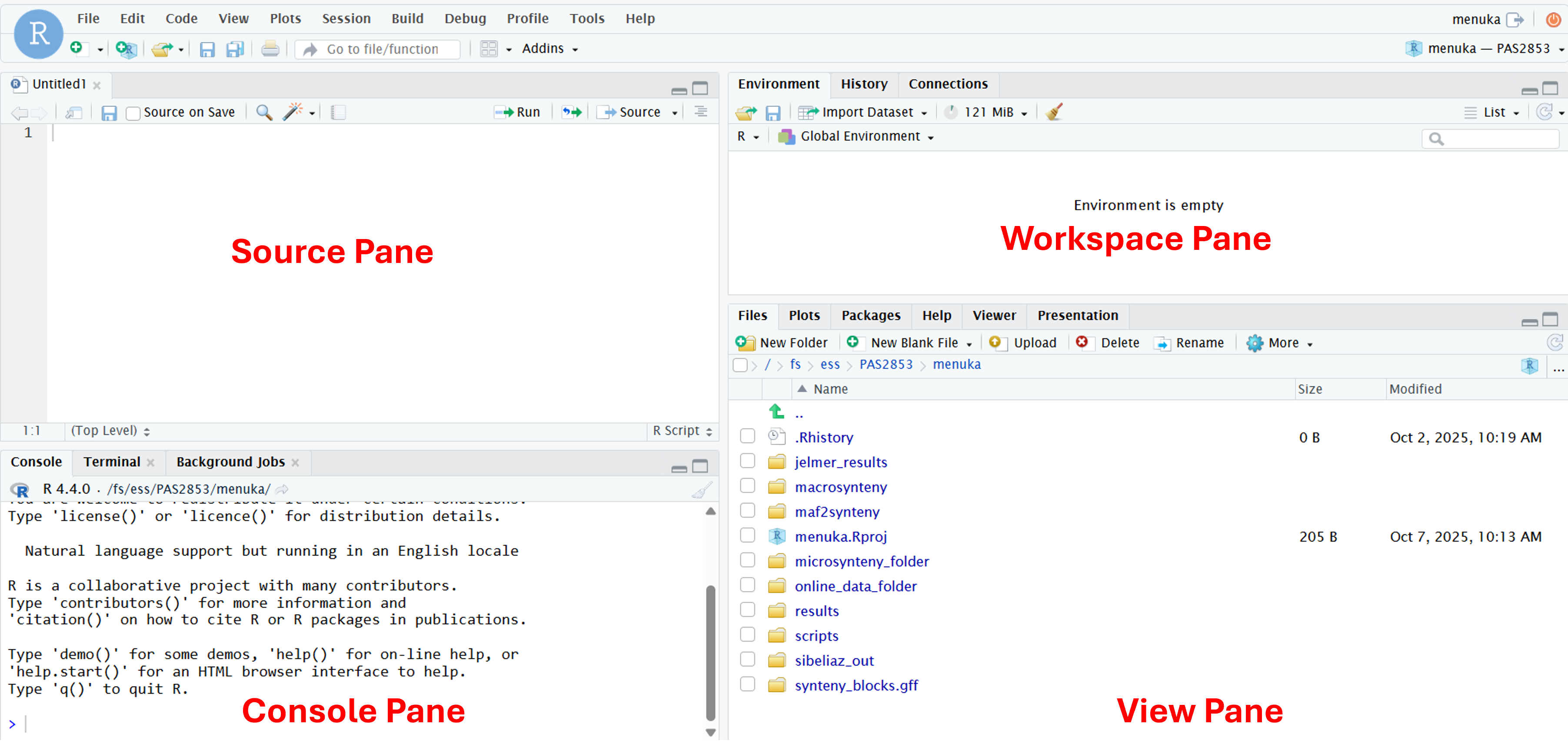
3 Orienting to RStudio (basic layout)

When you first open RStudio, you will be greeted by four panes, each of which have multiple tabs:

Top left: The editor/source pane, where you can open and edit documents like scripts
Bottom left: the default and most useful tab in this pane is your R “Console”, where you can type and execute R code
Top right: the default and most useful tab in this pane this is your “Environment”, which shows you all the objects that are active in your R environment
Bottom right: the default tab in this pane is “Files”, which is a file explorer starting in your initial working directory (more about that next). The additional tabs are also commonly used, such as those to show plots and help.

Click here for a useful RStudio cheatsheet

4 R basics

There are many things we can do in R: data manipulation, data visualization, statistical analysis, machine learning and many more. Here, to get some familiarity with working in R, we will start by simply using R as calculator.

4.1 R as calculator

To get used to typing and executing R code, we will simply use R as a calculator – type 5 + 5 in the console and press Enter:

5 + 5

[1] 10

R will print the result of the calculation, 10. The result is prefaced by [1], which is simply an index/count of output, which can be helpful when multiple numbers and elements are printed.

Some additional calculation examples:

Multiplication and division:
```
6 * 8
```
```
[1] 48
```
```
40 / 5
```
```
[1] 8
```
Exponents:
```
3 ^ 4
```
```
[1] 81
```

Parentheses can be used to change the default order of operations:

(5 + 3) * 2

[1] 16

# Without parentheses, multiplication happens first
5 + 3 * 2

[1] 11

These codes will work with (like shown above) or without spaces between numbers and around operators like +. However, in general, it is good practice to leave space between the number to improve the readability of your code.

Order of operations is as you learned in school (Click to expand)

When using R as a calculator, the order of operations is the same as you would have learned back in school. From highest to lowest precedence:

Parentheses: (, )
Exponents: ^ or **
Multiply: *
Divide: /
Add: +
Subtract: -

4.2 The R prompt

The > sign in your console is the R prompt, indicating that that R is ready for you to type something. In other words, this is equivalent to the $ Bash prompt that you are used to.

Also just like in Unix shell, when you are not seeing the > prompt, R is either busy (because you asked it to do a longer-running computation) or waiting for you to complete an incomplete command.

If you notice that your prompt turned into a +, you typed an incomplete command – for example:

10 /

And once again like in the Unix shell, you can either try to finish the command or abort it by pressing Ctrl+C. In R, Esc also works to cancel – let’s practice the latter here.

Adding comments to your code

Comments in R are just like in the Unix shell: you can use # signs to comment your code, both inline and on separate lines:

# This line is entirely ignored by R
10 / 5  # This line contains code but everything after the '#' is ignored

[1] 2

4.3 Comparing things

In R, you can use comparison operators to compare numbers. When you do this, R will return a so-called logical (one of R’s “data types” – more about these later): either FALSE or TRUE. For example:

Greater than and less than:
```
8 > 3
```
```
[1] TRUE
```
```
2 < 1
```
```
[1] FALSE
```

Equal to or not equal to – don’t forget to use two equals signs == for the former:

7 == 7

[1] TRUE

# The exclamation mark in general is a "negator"
10 != 5

[1] TRUE

Here are the most common comparison operators in R:

Operator	Description	Example
`>`	Greater than	5 > 6 returns `FALSE`
`<`	Less than	5 < 6 returns `TRUE`
`==`	Equal to	10 == 10 returns `TRUE`
`!=`	Not equal to	10 != 10 returns `FALSE`
`>=`	Greater than or equal to	5 >= 6 returns `FALSE`
`<=`	Less than or equal to	6 <= 6 returns `TRUE`

Exercise: R as a calculator

Find the natural log, log to the base 10, log to the base 2, square root and the natural antilog of 20.

Click to see a solution

To print log of 20 in different bases and square root and natural antilog of 20:

log(20)        # Natural log

[1] 2.995732

log10(20)     # Log to the base 10

[1] 1.30103

log2(20)      # Log to the base 2

[1] 4.321928

sqrt(20)      # Square root

[1] 4.472136

exp(20)       # Natural antilog

[1] 485165195

4.4 Functions in R

To do almost anything in R, you will use “functions”, which are the equivalent of Unix commands.

getwd()

/fs/ess/PAS2880/users

setwd("/fs/ess/PAS2880/users")

we need to quote /fs/ess/PAS2880/users because anything that is not quoted in R has to be object

list.files()

print("Hello world")

[1] "Hello world"

dir.create("week11")

Now, we will look at the head() function, which shows the first six rows of a data frame or matrix. We will use it to visualize the data sets present in R.

head(iris)

  Sepal.Length Sepal.Width Petal.Length Petal.Width Species
1          5.1         3.5          1.4         0.2  setosa
2          4.9         3.0          1.4         0.2  setosa
3          4.7         3.2          1.3         0.2  setosa
4          4.6         3.1          1.5         0.2  setosa
5          5.0         3.6          1.4         0.2  setosa
6          5.4         3.9          1.7         0.4  setosa

You can recognize function calls by parentheses. Inside those parentheses, you can provide arguments to a function. Arguments are the actual values you provided to run a function().

Arguments that are not object have to be in quotes in R

In R, you can choose to name the arguments in a function or just use their position, Named argument and positional argument. You can assign the values to argument, using the equal to sign =. When you assign values to the arguments, the order does not matter, R will know exactly which value goes where. For example, in head(n = 6, x = iris), the argument x is explicitly named so the function will run successfully. However, you can also write head(iris), and it gives the same output because R knows the first argument of head() is x. head(6, iris) will not produce any output because the arguments are called by position but are in the wrong order.

5 Functions in R

5.1 Basics of functions

To do almost anything in R, you will use “functions”, which are the equivalent of Unix commands. You can recognize function calls by the parentheses. For example:

The equivalent to the Shell’s pwd is getwd():
```
getwd()
```
```
/fs/ess/PAS2880/users
```
Inside those parentheses, you can provide arguments to a function. For example, using setwd(), the equivalent to the Shell’s cd:
```
setwd("/fs/ess/PAS2880/users")
```
Note that unlike in the Shell, we need to quote the path! This is because in R, as you’ll see in more detail in a bit, anything that is not quoted is supposed to be an “object” like a variable.
One of the equivalents to the Shell’s echo is print():
```
print("Hello world")
```
```
[1] "Hello world"
```
The equivalent to the Shell’s mkdir is dir.create():
```
dir.create("week11")
```

The equivalent to the Shell’s head is head(), although it will by default show 6 lines/rows instead of 10:

head(iris)

  Sepal.Length Sepal.Width Petal.Length Petal.Width Species
1          5.1         3.5          1.4         0.2  setosa
2          4.9         3.0          1.4         0.2  setosa
3          4.7         3.2          1.3         0.2  setosa
4          4.6         3.1          1.5         0.2  setosa
5          5.0         3.6          1.4         0.2  setosa
6          5.4         3.9          1.7         0.4  setosa

Where did iris come from?

R comes shipped with several built-in datasets, like iris. We didn’t need to (and shouldn’t) quote this, because it is a so-called object in R.

5.2 Function arguments

Consider the example below, where we pass the argument 6.53 to the function round():

round(6.53)

[1] 7

In most functions, including round(), arguments have names that can be used. For example, the argument to round() representing the number to be rounded has the name x, so you can also use:

round(x = 6.53)

[1] 7

Naming arguments is helpful in particular to avoid confusion when you pass multiple arguments to a function. For example, round() accepts a second argument, which is the number of digits to round to:

round(x = 6.53, digits = 1)

[1] 6.5

You could choose not to name these arguments, but that is not as easy to understand:

round(6.53, 1)

[1] 6.5

Moreover, when you name arguments, you can give them in any order you want:

round(digits = 1, x = 6.53)

[1] 6.5

You can usually see which arguments a function takes by pausing after your type the function and its parenthesis, e.g. round():

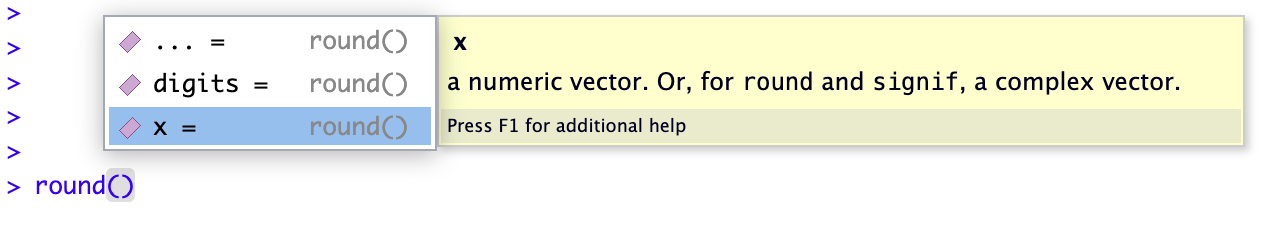
Below, we’ll also see more extensive options to find out how a function works and what arguments it takes.

5.3 Functions for everything

R has over 3,000 functions that serve many different purposes, and tens of thousands of additional functions are available in packages (add-ons). Below are a couple of examples continuing along the theme of using R as a calculator:

Function	Description
`abs(x)`	Absolute value: e.g. `abs(-5)` returns 5
`sqrt(x)`	Square root
`log(x)`	Natural logarithm
`log10(x)`	Common logarithm
`round(x, digits = n)`	Round: e.g `round(3.475, digits = 2)` returns 3.48

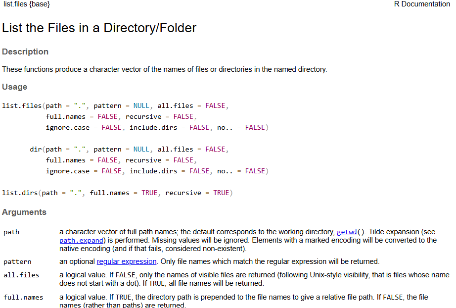
6 R Help: `help()` and `?`

The help() function and ? help operator in R offer access to documentation pages for R functions, data sets, and other objects. They provide access to both packages in the standard R distribution and contributed packages.

For example:

?list.files

The output should appear in the Viewer tab of the bottom-left panel in RStudio and should look something like this:

7 R objects

7.1 Assigning stuff to objects

You can assign one or more values to a so-called “object” with the assignment operator <-. A few examples:

# Assign the value 250 the object 'length_cm'
length_cm <- 250
length_cm

[1] 250

# Assign the value 2.54 to the object 'conversion'
conversion <- 2.54
conversion

[1] 2.54

In the shell, we’ve been calling these variables, and that terminology is also used for R objects like the above ones. However, R objects can take on many forms (we will talk about data structures in a bit), including more complicated things like tables. That’s why the general term object is used here.

To see the contents of an object, you can use the print() function as the equivalent of echo in the Unix shell:

print(length_cm)

[1] 250

However, in R you can also omit print() and simply type an object’s name:

length_cm

[1] 250

Importantly, you can use objects as if you had typed their values directly:

length_cm / conversion

[1] 98.4252

length_in <- length_cm / conversion
length_in

[1] 98.4252

7.2 Object names

Some pointers on object names:

Because R is case sensitive, length_inch is different from Length_Inch!
An object name cannot contain spaces — so for readability, you should separate words using:
- Underscores: length_inch (this is called “snake case”)
- Periods: wingspan.inch
- Capitalization: wingspanInch or WingspanInch (“camel case”)
You will make things easier for yourself by naming objects in a consistent way, for instance, by always sticking to your favorite case style like “snake case.”
Object names can contain but cannot start with a number: x2 is valid but 2x is not.
Make object names descriptive yet not too long — this is not always easy!

Exercise: Assigning objects in R

Write the R code to assign the value 20 to the name num_1 and 15 to num_2.
Click to see a solution
```
num_1 <- 20
num_2 <- 15
```

What is sum of num_1 and num_2?
Click to see a solution
```
num_1 + num_2
```
```
[1] 35
```

Assign the result of num_1 minus num_2 to a new object called difference. What is the value of difference?
Click to see a solution
```
difference <- num_1 - num_2
difference
```
```
[1] 5
```

Which of the following is a valid object name in R?
1. 2nd_value
2. value_2
3. total value
4. TotalValue
Click to see a solution

The valid object names are:
1. value_2
2. TotalValue
Object names cannot start with a number and cannot contain spaces (so a and c options are invalid).

8 R packages

R packages are basically add-ons or extensions to the functionality of the R language.

The function install.packages() installs an R package. This is a one-time operation, also at OSC (see below).
The function library() will load an R package in your current R session. Every time you want to use a package in R, you need to load it, just like everytime you want to use MS Word on your computer, you need to open it.

For example:

install.packages("stringr")

library(stringr)

install.packages("tidyverse")

# (Output like that shown below is expected if the package can be loaded:)
library(tidyverse)

── Attaching core tidyverse packages ──────────────────────── tidyverse 2.0.0 ──
✔ dplyr     1.1.4     ✔ purrr     1.1.0
✔ forcats   1.0.0     ✔ readr     2.1.5
✔ ggplot2   3.5.2     ✔ tibble    3.3.0
✔ lubridate 1.9.4     ✔ tidyr     1.3.1
── Conflicts ────────────────────────────────────────── tidyverse_conflicts() ──
✖ dplyr::filter() masks stats::filter()
✖ dplyr::lag()    masks stats::lag()
ℹ Use the conflicted package (<http://conflicted.r-lib.org/>) to force all conflicts to become errors

In RStudio server at OSC, packages will by default be installed into a standard location in your Home directory, so they can be accessed through time and regardless of what your working directory is, or what OSC project you are using¹.

However, package installation is done separately for:

Different major versions of R (e.g. 4.1 versus 4.2, but not R 4.1.1 versus 4.1.5). Therefore, when you switch to a different R version, you will start over with package installation².
Each OSC cluster, like Pitzer versus Cardinal.

9 Working directory and RStudio Projects

As shown earlier, you can figure out what your working directory is with getwd(), and change it with setwd().

However, there is a better way of dealing with working directories, which is to avoid using setwd() altogether and to use RStudio Projects instead. This is similar to the Open Folder functionality of VS Code, but then a bit more formalized.

RSudio projects are useful for several reasons:

Automatically manage your working directory : RStudio treats project folder as a working directory, thus there is no need of manually setting working directory
Keep you work organized : Organize your project inside self-contained folders, which helps to manage, share and reproduce results
Ensure clean R sessions : Switching projects will restart R and remove all the objects and loaded packages
Easy to collaborate : All the paths in the RSudio projects will be in relative to the project folder. So, your code will work without modification.

To create a new RStudio Project inside your personal dir in /fs/ess/PAS2880:

Click File (top bar, below your browser’s address bar) > New Project
In the popup window, click Existing Directory.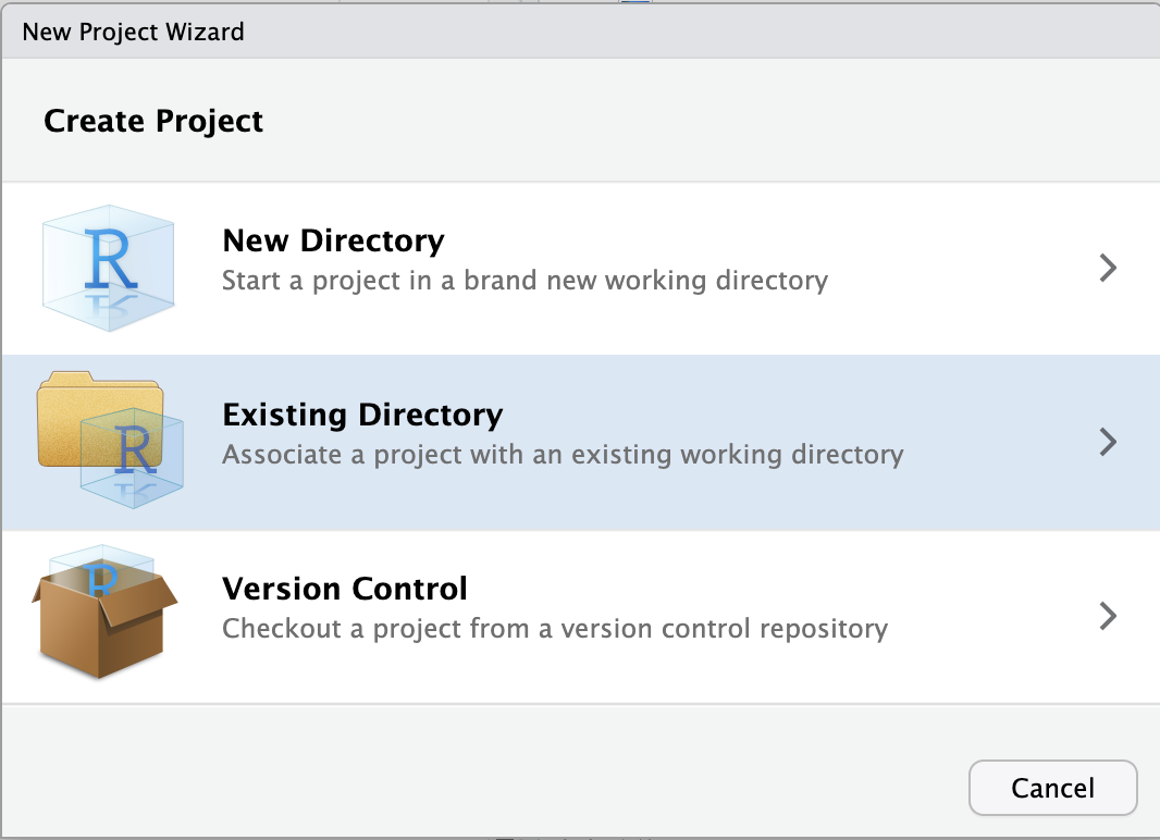

Click to see a screenshot

Click Browse... to select your personal dir.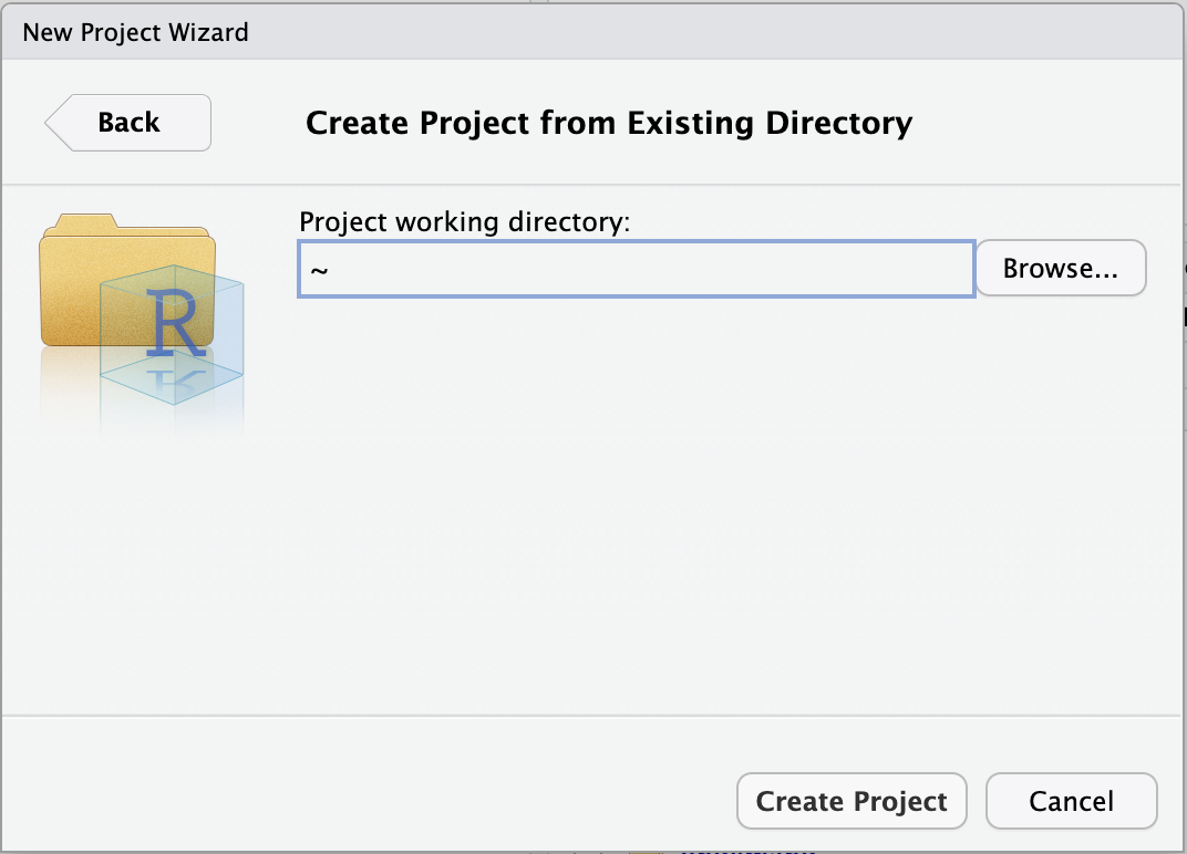

Click to see a screenshot

In the next window, you should be in your Home directory (abbreviated as ~), from which you can’t click your way to /fs/ess! Instead, you first have to click on the (very small!) ... highlighted in the screenshot below: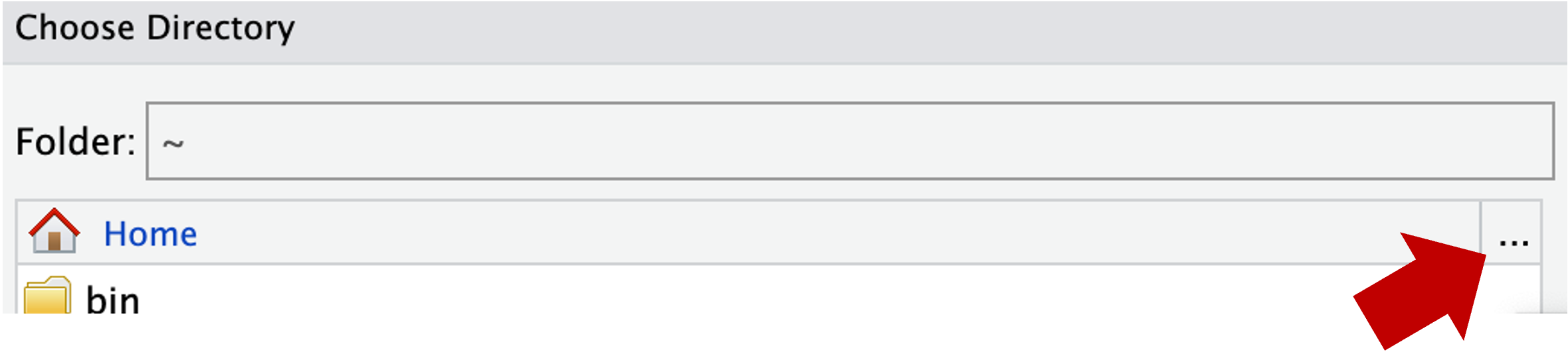

Type at least part of the path to your dir in /fs/ess/PAS2880, e.g. as shown below, and click OK::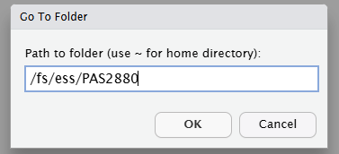

Now you should be able to browse/click the rest of the way to your dir (/fs/ess/PAS2880/users/$USER).
Click Choose to pick your selected directory.
Click Create Project.

This will make R restart, which is by design. When R restarts, all objects are removed from the environment, packages are unloaded, and so on. This is a good idea whenever you switch to a different project, for example to avoid irreproducible carry-over effects.

10 R scripts

Once you open a file, a new RStudio panel will appear in the top-left, where you can view and edit text files, most commonly R scripts (.R). An R script is a text file that contains R code.

Create and open a new R script by clicking File (top menu bar) > New File > R Script.

Why use a script?

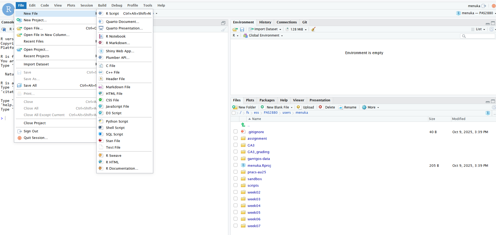
It’s a good idea to write and save most of your code in scripts, instead of directly in the R console. This helps to keep track of what you’ve been doing, especially in the longer run, and to re-run your code after modifying input data or one of the lines of code.

Sending code to the console

To send code from the editor to the console, where it will be executed by R, press Ctrl + Enter (or, on a Mac: Cmd + Enter) with the cursor anywhere in a line of code in the script.

Practice that after typing the following command in the script:

5 + 5

[1] 10

11 Recap and looking forward

R Objects : Restore and use data.
Arguments of Function : Use R packages and write our own function.
R Packages : Install and load various useful packages for analysis.
R Projects : Reproducibility and keep your work structured.
R script : Document workflow for future use.

References

Garrigós, Marta, Guillem Ylla, Josué Martínez-de la Puente, Jordi Figuerola, and María José Ruiz-López. 2025. “Two Avian Plasmodium Species Trigger Different Transcriptional Responses on Their Vector Culex pipiens.” Molecular Ecology 34 (15): e17240. https://doi.org/10.1111/mec.17240.

Footnotes

And this works equivalently on your own computer.↩︎
This too, works the same with R on your own computer.↩︎