One of R’s most powerful features is its built-in ability to deal with tabular data – i.e., data with rows and columns like you are familiar with from Excel spreadsheets and so on. In R, tabular data is stored in a data structure called “data frame”.
In this lecture, you will learn:
Data frames and different functions to reorganize and modify data frames
Open a new R Script and save it as week11c.R in your week11 folder (R scripts)
2 The tidyverse
We’ll start working with a family of R packages designed for “dataframe-centric” data science called the “tidyverse”. Dataframe-centric refers to doing most if not all data analysis while keeping the data in R’s data frame data structure.
All core tidyverse packages can be installed and loaded with a single command. Since you should already have installed the tidyverse1, you only need to load it, which you do as follows:
library(tidyverse)
── Attaching core tidyverse packages ──────────────────────── tidyverse 2.0.0 ──
✔ dplyr     1.1.4     ✔ readr     2.1.5
✔ forcats   1.0.0     ✔ stringr   1.5.2
✔ ggplot2   3.5.2     ✔ tibble    3.3.0
✔ lubridate 1.9.4     ✔ tidyr     1.3.1
✔ purrr     1.1.0
── Conflicts ────────────────────────────────────────── tidyverse_conflicts() ──
✖ dplyr::filter() masks stats::filter()
✖ dplyr::lag()    masks stats::lag()
ℹ Use the conflicted package (<http://conflicted.r-lib.org/>) to force all conflicts to become errors
The output tells you which packages have been loaded as part of the tidyverse.
One thing to note about the tidyverse is that much of its functionality is also covered by base R functions, but it is better suited for quick and easy data manipulation.
Function name conflicts (Click to expand)
When you loaded the tidyverse, the output included a “Conflicts” section that may have seemed ominous:
── Conflicts ────────────────────────────────────────── tidyverse_conflicts() ──
✖ dplyr::filter() masks stats::filter()
✖ dplyr::lag()    masks stats::lag()
ℹ Use the conflicted package (<http://conflicted.r-lib.org/>) to force all conflicts to become errors
What this means is that two tidyverse functions, filter() and lag(), have the same names as two functions from the stats package that were already in your R environment.
Those stats package functions are part of what is often referred to as “base R”: core R functionality that is always available (loaded) when you start R.
Due to this function name conflict/collision, the filter() function from dplyr “masks” the filter() function from stats. Therefore, if you write a command with filter(), it will use the dplyr function and not the stats function.
You can use a “masked” function, by prefacing it with its package name as follows: stats::filter().
3 Reading data
readr is one of the packages that is loaded as part of the core tidyverse, and has functions for reading and writing tabular data to and from plain-text files like CSV and TSV files.
The read_tsv() function will read TSV (tab-delimited files) – for example:
meta <-read_tsv(file ="garrigos-data/meta/metadata.tsv")
Rows: 22 Columns: 3
── Column specification ────────────────────────────────────────────────────────
Delimiter: "\t"
chr (3): sample_id, time, treatment

ℹ Use `spec()` to retrieve the full column specification for this data.
ℹ Specify the column types or set `show_col_types = FALSE` to quiet this message.
Note that this function is rather chatty, telling you how many rows and columns it read, and what their data types are. Let’s check the resulting object:
meta
# A tibble: 22 × 3
   sample_id   time  treatment
   <chr>       <chr> <chr>
 1 ERR10802882 10dpi cathemerium
 2 ERR10802875 10dpi cathemerium
 3 ERR10802879 10dpi cathemerium
 4 ERR10802883 10dpi cathemerium
 5 ERR10802878 10dpi control
 6 ERR10802884 10dpi control
 7 ERR10802877 10dpi control
 8 ERR10802881 10dpi control
 9 ERR10802876 10dpi relictum
10 ERR10802880 10dpi relictum
# ℹ 12 more rows
To read and write CSV files instead, use read_csv() / write_csv() in the same way.
You can also use the View() function to look at the data frame. This will open a new tab in your editor pane with a spreadsheet-like look and feel:
View(meta)# (Should display the dataset in an editor pane tab)
4 Data frame basics
Data frames are another R data structure, like vectors.
They contain tabular data and can be thought of a vectors pasted side-by-side: each column is a vector. This means that each column can only contain one data type.
It also implies that rows and columns aren’t equivalent. Specifically, it is good practice to organize tabular data in the so-called “tidy” data format like above, where:
Each column contains a different “variable” (e.g. coat color, weight)
Each row contains a different “observation” (data on e.g. one cat/person/sample)
… a so-called “tibble”, which is the tidyverse variant of a data frame. The main difference is the nicer default printing behavior of tibbles: e.g. the data types of columns are shown, and only a limited number of rows are printed.
4.1 Extracting columns from a data frame
You can extract individual columns from a data frame using the $ operator:
This kind of operation will return a vector – and can be indexed as well:
meta$treatment[2]
[1] "cathemerium"
5 Matrices
The matrix data structure in R is similar to a data frame: it is also rectangular with rows and columns. But it differs in that all the elements in a matrix must of be same data type: all numeric, character, or logical. This restriction applies only to the contents of the matrix which is the actual numbers inside the rectangular data area. However, rownames and colnames are not part of the matrix’s main data content. They are attributes attached to the matrix object.
Most commonly, matrices consist of only numerical data.
Of course, column labels can then still be provided with column names, but what about rows?
Rownames are typically used for feature IDs (e.g., genes) in Matrix and column names represent sample_ID. These rownames are important for RNAseq data analysis package DESeq2 because the software uses rownames to match genes across the count matrix and associated metadata. While data frames in R also allow rownames, they are less commonly used for storing identifiers like gene names. Instead, genes names are usually stored as a separate column for clarity in data frame.
Generally, matrices are not nearly as common as data frames, but we are introducing them here because they are used in a number of omics-data related packages. For example, the package DESeq2, which we’ll later use for differential expression analysis of our RNA-Seq count data.
6 The dplyr package
The dplyr package provides very useful functions for manipulating data in data frames (“data wrangling”). This type of data processing is often essential before you can move on to say, data visualization (week 13) or statistical data analysis (week 14).
In this session, we’ll cover the most commonly used dplyr functions:
select() to pick columns (variables)
filter() to pick rows (observations)
rename() to change column names
arrange() to change the order of rows (i.e., to sort a data frame)
mutate() to modify values in columns and create new columns
summarize() to compute across-row summaries
All these functions take a data frame as the input, and output a new, modified data frame.
7select() to pick columns (variables)
The first dplyr function you’ll learn about is select(), which subsets a data frame by including/excluding certain columns. By default, it only includes the columns you specify:
Above, the first argument was the data frame, whereas the other arguments were the (unquoted!) names of columns to be included in the output data frame2.
The order of the columns in the output data frame is exactly as you list them in select(), and doesn’t need to be the same as in the input data frame. In other words, select() is also one way to reorder columns: in the example above, we made year appear before country.
You can also specify columns that should be excluded, by prefacing their name with a ! (or a -):
# This will include all columns _except_ sample_id:select(.data = meta, !sample_id)
# A tibble: 22 × 2
   time  treatment
   <chr> <chr>
 1 10dpi cathemerium
 2 10dpi cathemerium
 3 10dpi cathemerium
 4 10dpi cathemerium
 5 10dpi control
 6 10dpi control
 7 10dpi control
 8 10dpi control
 9 10dpi relictum
10 10dpi relictum
# ℹ 12 more rows
There are also ways to e.g. select ranges of columns: check the select() help by typing ?select to learn more.
8rename() to change column names
The next dplyr function is one of the simplest: rename() to change column names.
The syntax to specify the new and old name within the function is new_name = old_name. For example:
rename(.data = meta, sample = sample_id)
# A tibble: 22 × 3
   sample      time  treatment
   <chr>       <chr> <chr>
 1 ERR10802882 10dpi cathemerium
 2 ERR10802875 10dpi cathemerium
 3 ERR10802879 10dpi cathemerium
 4 ERR10802883 10dpi cathemerium
 5 ERR10802878 10dpi control
 6 ERR10802884 10dpi control
 7 ERR10802877 10dpi control
 8 ERR10802881 10dpi control
 9 ERR10802876 10dpi relictum
10 ERR10802880 10dpi relictum
# ℹ 12 more rows
9 The pipe (|>)
Examples so far applied a single dplyr function to a data frame, simply printing the output (a new data frame) to screen. But in practice, it’s common to use several consecutive dplyr functions to wrangle a dataframe into the format you want.
For example, you may want to first select() one or more columns, and thenrename() a column. You could do that as follows:
And you could go on along these lines, successively creating new objects that you then use for the next step.
But there is a more elegant way of dong this, directly sending (“piping”) output from one function into the next function with the pipe operator|> (a vertical bar | followed by a greater-than sign >). Let’s start by seeing a reformulation of the code above with pipes:
meta |>select(sample_id, time) |>rename(sample = sample_id)
What happened here? We took the meta data frame, sent (“piped”) it into the select() function, whose output in turn was piped into the rename() function. You can think of the pipe as “then”: take meta, then select, then rename.
When using the pipe, you no longer specify the input data frame with the .data argument, because the function now gets its input data via the pipe (specifically, the input goes to the function’s first argument by default).
Using pipes involves less typing and is especially more readable than using successive assignments3.
For code readability, it is good practice to always start a new line after a pipe |>, and to keep the subsequent line(s) indented as RStudio will automatically do.
Using the pipe keyboard shortcut
The following RStudio keyboard shortcut will insert a pipe symbol: Ctrl/Cmd + Shift + M.
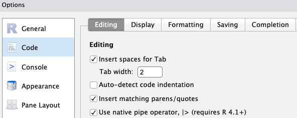
However, by default this (still) inserts an older pipe symbol, %>%. As long as you’ve loaded the tidyverse4, it would not really be a problem to just use %>% instead of |>. But it would be preferred to make RStudio insert the |> pipe symbol:
Click Tools > Global Options > Code tab on the right
Check the box “Use native pipe operator” as shown below
Click OK at the bottom of the options dialog box to apply the change and close the box.
10filter() to pick rows (observations)
10.1 Introduction
The filter() function outputs only those rows that satisfy one or more conditions. It is similar to Filter functionality in Excel – except that those only change what you display, while filter() will completely exclude rows.
But if that sounds scary, recall that dplyr functions always output a new data frame. Therefore, with any dplyr function, you’ll only modify existing data when you assign the output back to the input object, like in this example with the select() function:
# [Don't run this - hypothetical example]# After running this, the 'meta' dataframe would no longer contain the treatment column:meta <- meta |>select(sample_id, time)
10.2 Filter based on one condition
This first filter() example outputs only rows with the sampling time point 10dpi (remember, each row of time variable represents a sample at a given time point):
meta |>filter(time =="10dpi")
# A tibble: 12 × 3
   sample_id   time  treatment
   <chr>       <chr> <chr>
 1 ERR10802882 10dpi cathemerium
 2 ERR10802875 10dpi cathemerium
 3 ERR10802879 10dpi cathemerium
 4 ERR10802883 10dpi cathemerium
 5 ERR10802878 10dpi control
 6 ERR10802884 10dpi control
 7 ERR10802877 10dpi control
 8 ERR10802881 10dpi control
 9 ERR10802876 10dpi relictum
10 ERR10802880 10dpi relictum
11 ERR10802885 10dpi relictum
12 ERR10802886 10dpi relictum
How many rows were output? (Click to see the answer)
21 rows were output, as shown in the first line above: 12 x 3 (rows x columns)
Remember to use two equals signs == to test for equality!
10.3 Filter based on multiple conditions
It’s also possible to filter based on multiple conditions. For example, you may want to see control samples collected at 10dpi excluding ERR10802882:
meta |>filter(time =="10dpi", treatment =="control", sample_id !="ERR10802882")
# A tibble: 4 × 3
  sample_id   time  treatment
  <chr>       <chr> <chr>
1 ERR10802878 10dpi control
2 ERR10802884 10dpi control
3 ERR10802877 10dpi control
4 ERR10802881 10dpi control
Like above, by default, multiple conditions are combined using a Boolean AND. In other words, in a given row, each condition must be met to output the row.
If you want to combine conditions using a Boolean OR, where only one of the conditions needs to be met, use a | between the conditions:
# Keep rows with a control samples collected at 10dpi:meta |>filter(time =="10dpi"| treatment =="control")
# A tibble: 15 × 3
   sample_id   time  treatment
   <chr>       <chr> <chr>
 1 ERR10802882 10dpi cathemerium
 2 ERR10802875 10dpi cathemerium
 3 ERR10802879 10dpi cathemerium
 4 ERR10802883 10dpi cathemerium
 5 ERR10802878 10dpi control
 6 ERR10802884 10dpi control
 7 ERR10802877 10dpi control
 8 ERR10802881 10dpi control
 9 ERR10802876 10dpi relictum
10 ERR10802880 10dpi relictum
11 ERR10802885 10dpi relictum
12 ERR10802886 10dpi relictum
13 ERR10802866 24hpi control
14 ERR10802869 24hpi control
15 ERR10802863 24hpi control
10.4 Pipeline practice
Finally, let’s practice once more with “pipelines” that use multiple dplyr functions: filter rows, then select columns, and finally rename one of the remaining columns:
meta |>filter(time =="10dpi") |>select(sample_id, treatment) |>rename(sample = sample_id)
# A tibble: 12 × 2
   sample      treatment
   <chr>       <chr>
 1 ERR10802882 cathemerium
 2 ERR10802875 cathemerium
 3 ERR10802879 cathemerium
 4 ERR10802883 cathemerium
 5 ERR10802878 control
 6 ERR10802884 control
 7 ERR10802877 control
 8 ERR10802881 control
 9 ERR10802876 relictum
10 ERR10802880 relictum
11 ERR10802885 relictum
12 ERR10802886 relictum
Exercise: Pipes
Use a “pipeline” like above to output a data frame with two columns (sample_id and treatment) only for the cathemerium treatment. How many rows does your output data frame have?
Click for the solution
meta |>select(sample_id, treatment) |>filter(treatment =="cathemerium")
The arrange() function is like sorting functionality in Excel: it changes the order of rows based on the values in one or more columns5. Among other things, sorting can help you find observations with the smallest or largest values for a certain column.
The meta dataframe is currently first sorted by time and then by treatment, whereas sample_ids within these groups are not sorted. You may, for example, want to sort by sample_id instead:
meta |>arrange(sample_id)
# A tibble: 22 × 3
   sample_id   time  treatment
   <chr>       <chr> <chr>
 1 ERR10802863 24hpi control
 2 ERR10802864 24hpi cathemerium
 3 ERR10802865 24hpi relictum
 4 ERR10802866 24hpi control
 5 ERR10802867 24hpi cathemerium
 6 ERR10802868 24hpi relictum
 7 ERR10802869 24hpi control
 8 ERR10802870 24hpi cathemerium
 9 ERR10802871 24hpi relictum
10 ERR10802874 24hpi relictum
# ℹ 12 more rows
Default sorting is alphabetically and, for numbers, from small to large. To sort in reverse order, use the desc() (descending) helper function:
meta |>arrange(desc(sample_id))
# A tibble: 22 × 3
   sample_id   time  treatment
   <chr>       <chr> <chr>
 1 ERR10802886 10dpi relictum
 2 ERR10802885 10dpi relictum
 3 ERR10802884 10dpi control
 4 ERR10802883 10dpi cathemerium
 5 ERR10802882 10dpi cathemerium
 6 ERR10802881 10dpi control
 7 ERR10802880 10dpi relictum
 8 ERR10802879 10dpi cathemerium
 9 ERR10802878 10dpi control
10 ERR10802877 10dpi control
# ℹ 12 more rows
Finally, you may want to sort by multiple columns, where ties in the first column are broken by a second column (and so on). Do this by simply listing the columns in the appropriate order:
# Sort first by treatment, time, then by sample_id:meta |>arrange(treatment, time, sample_id)
# A tibble: 22 × 3
   sample_id   time  treatment
   <chr>       <chr> <chr>
 1 ERR10802875 10dpi cathemerium
 2 ERR10802879 10dpi cathemerium
 3 ERR10802882 10dpi cathemerium
 4 ERR10802883 10dpi cathemerium
 5 ERR10802864 24hpi cathemerium
 6 ERR10802867 24hpi cathemerium
 7 ERR10802870 24hpi cathemerium
 8 ERR10802877 10dpi control
 9 ERR10802878 10dpi control
10 ERR10802881 10dpi control
# ℹ 12 more rows
12mutate() to modify columns and create new ones
So far, we’ve focused on functions that subset and reorganize data frames (and you’ve seen how to modify column names). But you haven’t seen how you can change the data or compute derived data.
You can do this with the mutate() function. For a first example, let’s go back to the iris dataframe:
Both data frames and tibbles are used in R to store tabular data containing rows and columns, often with mixed data types (character, integer, double etc).
Data frames : Introduced in base R, available without loading any package. Often convert character data into factors automatically (though this can be disabled with stringsAsFactors = FALSE). Print all rows and columns by default, which can be overwhelming for large datasets. When subsetting, R may simplify results unexpectedly (e.g., returning a vector instead of a data frame).
Tibbles : Tibbles are data frames, but they tweak some older behaviors to make life a little easier. Introduced in the tidyverse (specifically, the tibble package), and are part of the tidyverse ecosystem. Do not automatically convert strings to factors — everything stays as you enter it. Print in a more readable way, showing only the first 10 rows and all columns that fit on the screen. When subsetting, tibbles always return another tibble, preserving the data frame structure (unless you explicitly ask for it).
For an example with our meta dataframe, we’ll use the sub() function, which can do a character-based search-and-replace. It takes three arguments: the pattern to search for, what to replace the pattern with, and the subject vector. For example, to shorten sample IDs by removing the shared prefix:
# Create a new column 'sample_id_short' by replacing the 'ERR10802' pattern of sample_id with nothing :meta |>mutate(sample_id_short =sub(pattern ="ERR10802", replacement ="", x = sample_id) )
# A tibble: 22 × 4
   sample_id   time  treatment   sample_id_short
   <chr>       <chr> <chr>       <chr>
 1 ERR10802882 10dpi cathemerium 882
 2 ERR10802875 10dpi cathemerium 875
 3 ERR10802879 10dpi cathemerium 879
 4 ERR10802883 10dpi cathemerium 883
 5 ERR10802878 10dpi control     878
 6 ERR10802884 10dpi control     884
 7 ERR10802877 10dpi control     877
 8 ERR10802881 10dpi control     881
 9 ERR10802876 10dpi relictum    876
10 ERR10802880 10dpi relictum    880
# ℹ 12 more rows
The above examples added a new column to the dataframe. To modify an existing column rather than adding a new one, simply “assign back to the same name”:
meta |>mutate(sample_id =sub(pattern ="ERR10802", replacement ="", x = sample_id) )
# A tibble: 22 × 3
   sample_id time  treatment
   <chr>     <chr> <chr>
 1 882       10dpi cathemerium
 2 875       10dpi cathemerium
 3 879       10dpi cathemerium
 4 883       10dpi cathemerium
 5 878       10dpi control
 6 884       10dpi control
 7 877       10dpi control
 8 881       10dpi control
 9 876       10dpi relictum
10 880       10dpi relictum
# ℹ 12 more rows
Exercise: mutate()
Another very useful function is substr(), short for substring, which can extract parts of a character vector by position: say, you can ask it to only keep the first three characters. It includes arguments for the desired start and end positions of the substring:
meta |>mutate(treatment_short =substr(x = treatment, start =1, stop =3))
# A tibble: 22 × 4
   sample_id   time  treatment   treatment_short
   <chr>       <chr> <chr>       <chr>
 1 ERR10802882 10dpi cathemerium cat
 2 ERR10802875 10dpi cathemerium cat
 3 ERR10802879 10dpi cathemerium cat
 4 ERR10802883 10dpi cathemerium cat
 5 ERR10802878 10dpi control     con
 6 ERR10802884 10dpi control     con
 7 ERR10802877 10dpi control     con
 8 ERR10802881 10dpi control     con
 9 ERR10802876 10dpi relictum    rel
10 ERR10802880 10dpi relictum    rel
# ℹ 12 more rows
Use mutate() with substr() to:
Create a numeric time_num column, stripping the hpi/dpi suffix from time.
Create a column time_unit, keeping only the hpi/dpi suffix from time.
Save the resulting data frame as meta_time (we will use it after this!).
The final function dplyr function we’ll cover is summarize(), which computes summaries of your data across rows. For example, to calculate the mean time across the entire dataset (all rows):
# The syntax is similar to 'mutate': <new-column> = <operation>meta_time |>summarize(mean_time =mean(time_num))
# A tibble: 1 × 1
  mean_time
      <dbl>
1      16.4
The output is still a dataframe, but unlike with all previous dplyr functions, it is completely different from the input dataframe, “collapsing” the data down to as little as a single number, like above.
summarize() becomes really powerful in combination with the helper function group_by() to compute groupwise stats. For example, to get the mean time_num separately for each treatment:
# A tibble: 3 × 2
  treatment   mean_time
  <chr>           <dbl>
1 cathemerium        16
2 control            16
3 relictum           17
group_by() implicitly splits a data frame into groups of rows: here, one group for observations from each treatment. After that, operations like in summarize() will happen separately for each group, which is how we ended up with per-treatment means.
Before doing the exercise for summarize(), we will learn about the new function str() to understand the internal structure of your dataset/object. The argument for the str() is the name of the object you want to explore.
To write a data frame to a TSV file, you can use the write_tsv() function, with argument x for the R object and argument file for the file path:
# You can save in the present working directory write_tsv(x = meta_time, file ="metadata_ed.tsv")# Change the path if you want to save it in different directorywrite_tsv(x = meta_time, file ="results/metadata_ed.tsv")
Because we simply provided a file name, the file will have been written in your R working directory6.
If you want to take a look at the file you just created, you can find it in RStudio’s Files tab and click on it, which will open it in the editor panel. Of course, you could also find it in your computer’s file browser and open it in different ways.
15 Recap and looking forward
Different columns of Data frame can contain different types of data, but in a matrix all the elements are of same data type.
Several functions of dplyr package such as filter(), select(), arrange(), mutate() in R provides a powerful way to manipulate large datasets.
Learn more
Regarding data wrangling specifically, here are two particularly useful additional skills to learn:
Pivoting/reshaping — moving between ‘wide’ and ‘long’ data formats with pivot_wider() and pivot_longer(). This is covered in chapter 5 of R for Data Science.
Joining/merging — combining multiple dataframes based on one or more shared columns. This can be done with dplyr’s join_*() functions – see for example chapter 19 of R for Data Science.
Based on what you learned in the previous session, it may seem strange that the column names should not be quoted. One way to make sense of this is that the columns can be thought of as (vector) objects, whose names are the column names.↩︎
Using pipes is also faster and uses less computer memory.↩︎
This symbol only works when you have one of the tidyverse packages loaded.↩︎
It will always rearrange the order of rows as a whole, never just of individual columns since that would scramble the data.↩︎
Recall that you can see where that is at the top of the Console tab, or by running getwd().↩︎