Omics Data
With a focus on high-throughput sequencing data
2025-08-26
The main omics data types
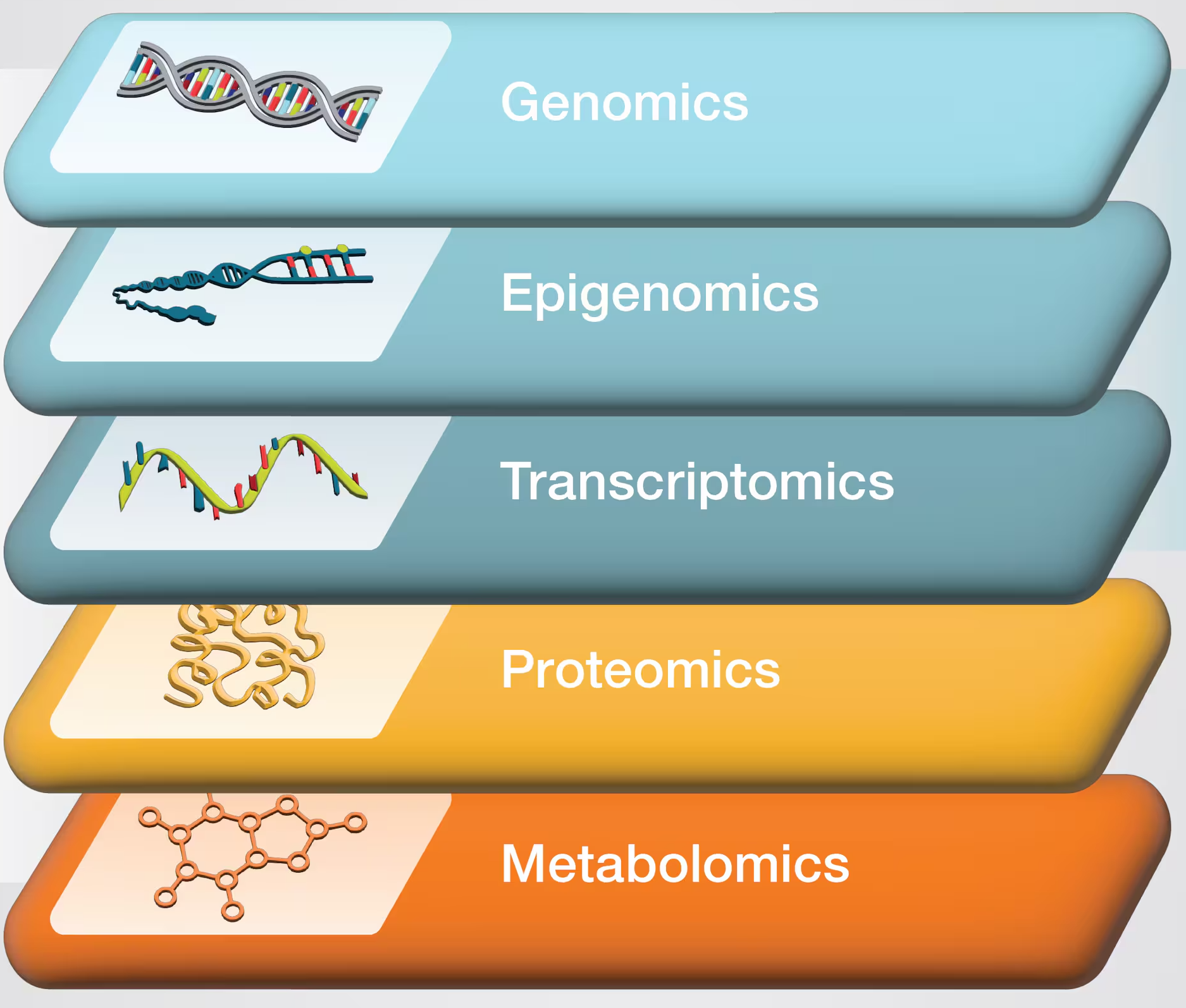
Copyright ThermoFisher
Learn more in this week’s first reading
Poinsignon et al. (2023): Working with omics data: An interdisciplinary challenge at the crossroads of biology and computer science
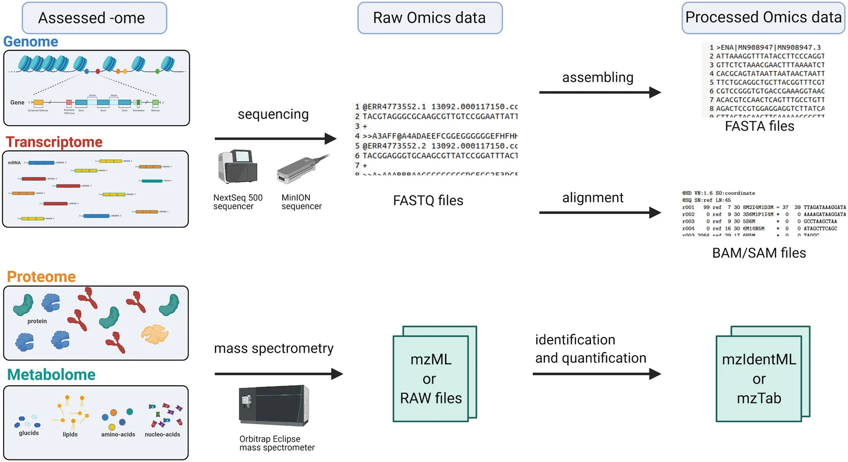
Figure 2 from the paper.
Libraries and library prep
In a sequencing context, a “library” is a collection of nucleic acid fragments ready for sequencing.
We’ll go into some specifics of Illumina library prep because this is the most common type of HTS, and we’ll use Illumina read files as examples throughout the course.
In Illumina and other HTS libraries, these fragments number in the millions or billions and are often simply randomly generated from input such as genomic DNA:
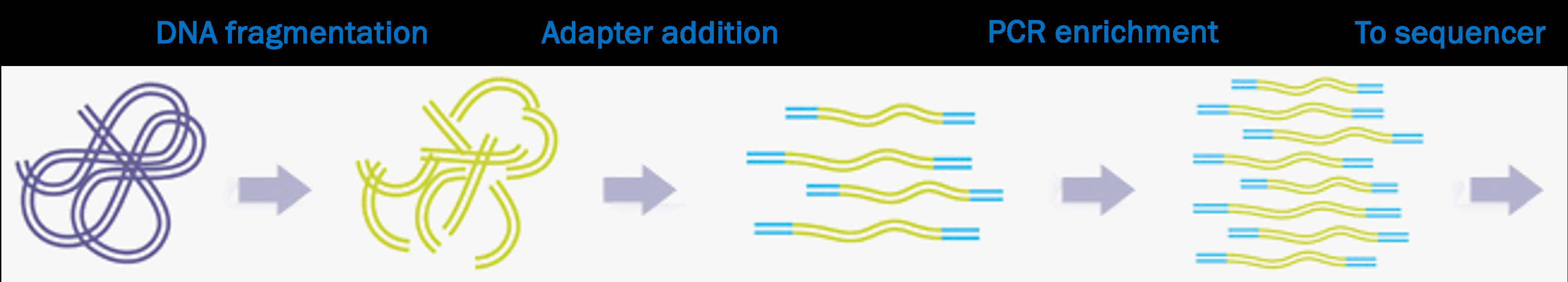
An overview of the library prep procedure. This is typically done for you by a sequencing facility or company.
A closer look at the processed DNA fragments
As shown in the previous slide, after library prep, each DNA fragment is flanked by several types of short sequences that together make up the “adapters”:

Multiplexing!
Adapters can include so-called “indices” or “barcodes” that identify individual samples. That way, up to 96 samples can be combined (multiplexed) into a single library, i.e. into a single tube.
Paired-end vs. single-end sequencing
DNA fragments can be sequenced from both ends as shown below —
this is called “paired-end” (PE) sequencing:

When sequencing is instead single-end (SE), no reverse read is produced:

Insert size variation
The DNA fragment’s size (“insert size” ) can vary – by design, but also because of limited precision in size selection. In some cases, it is:
Shorter than the combined read length, which leads to?
- Overlapping reads (this can be useful!):

Shorter than the single read length, which leads to?
- “Adapter read-through”: the final bases in the resulting reads will consist of adapter sequence, which should be removed before moving on.

Garrigós et al. 2025
Throughout the course, we’ll use an example/practice data set from Garrigós et al. (2025):
This paper uses paired-end Illumina RNA-Seq data to study gene expression in Culex pipiens mosquitos infected with two different malaria-causing Plasmodium protozoans.
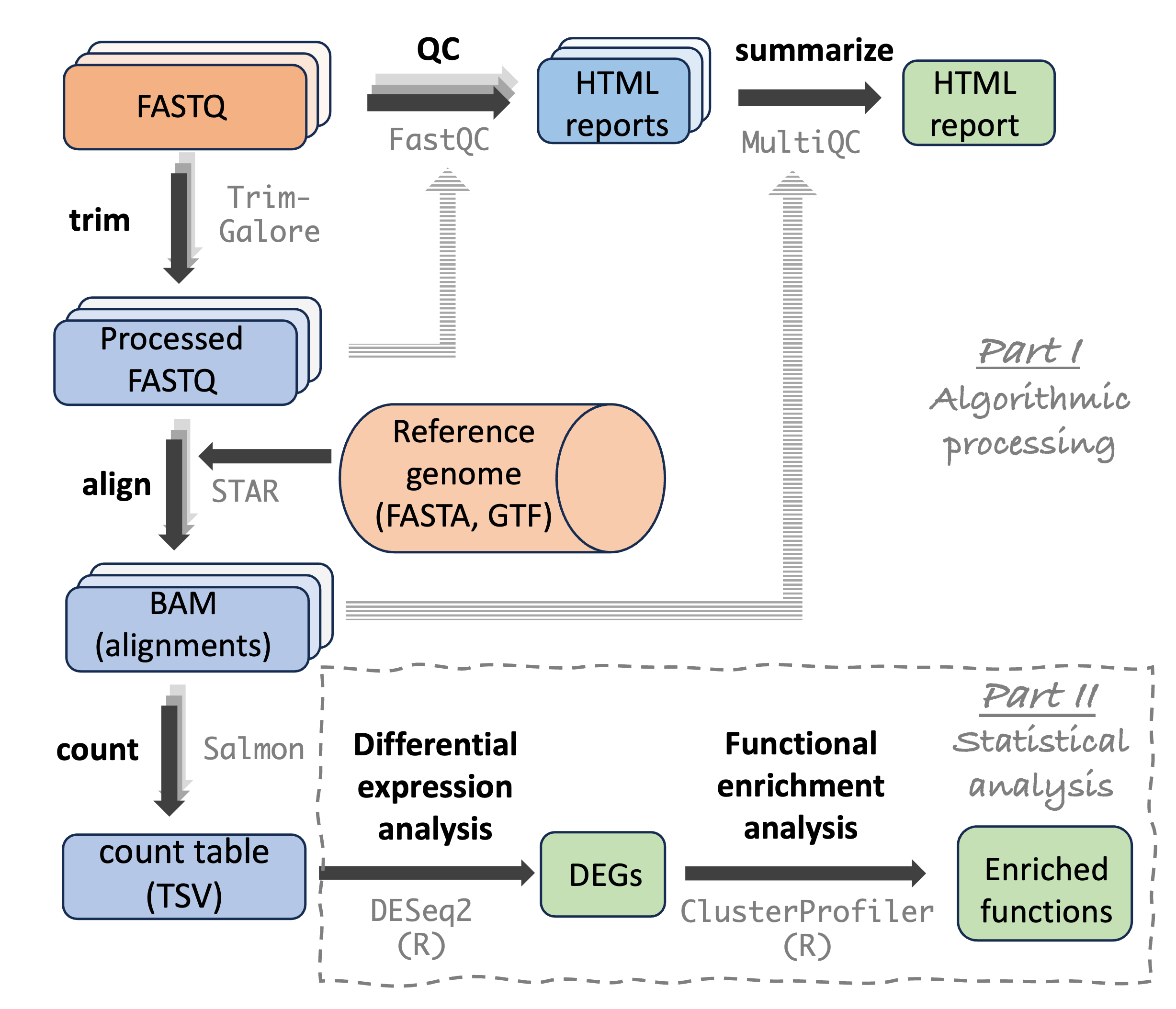
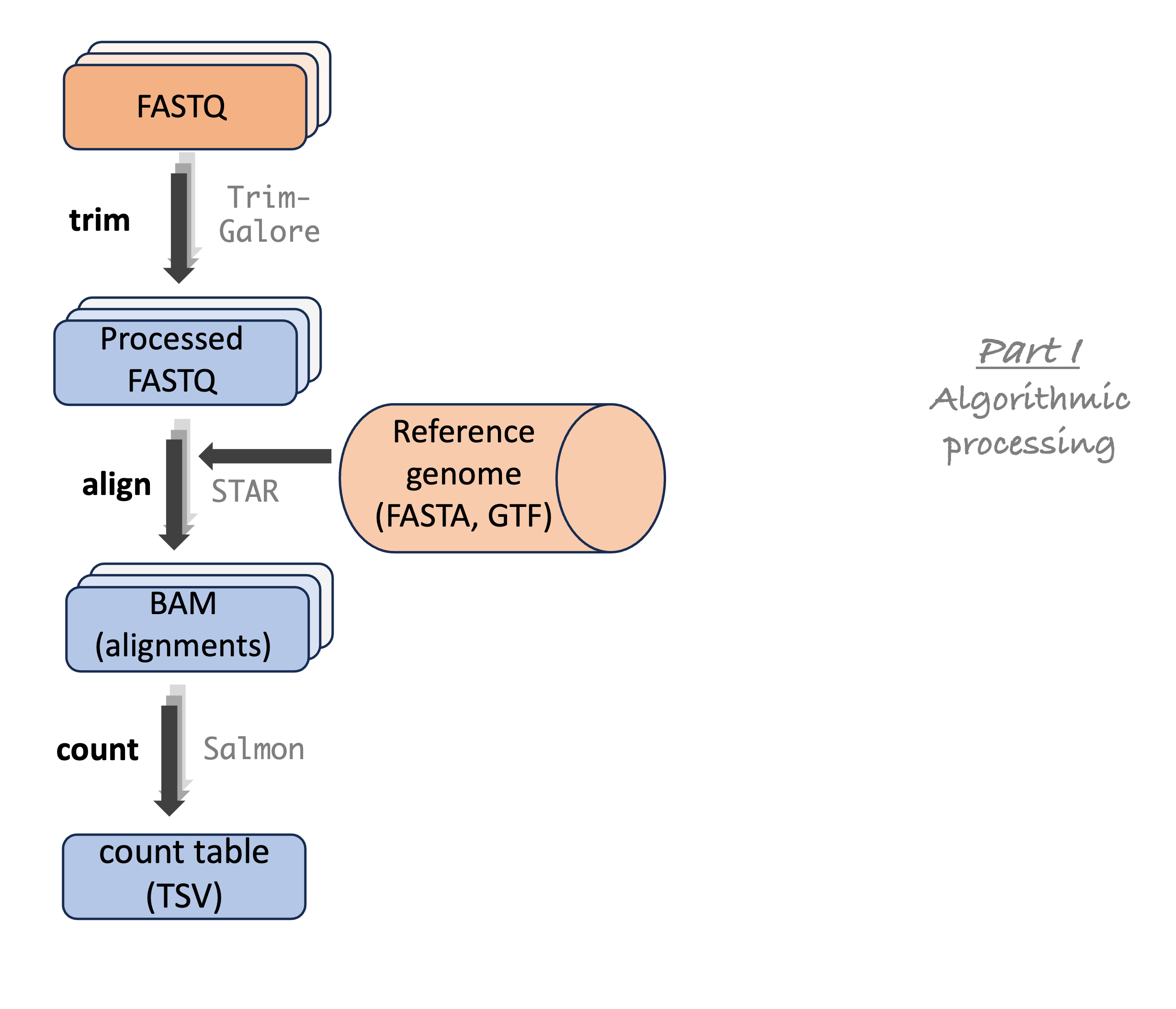
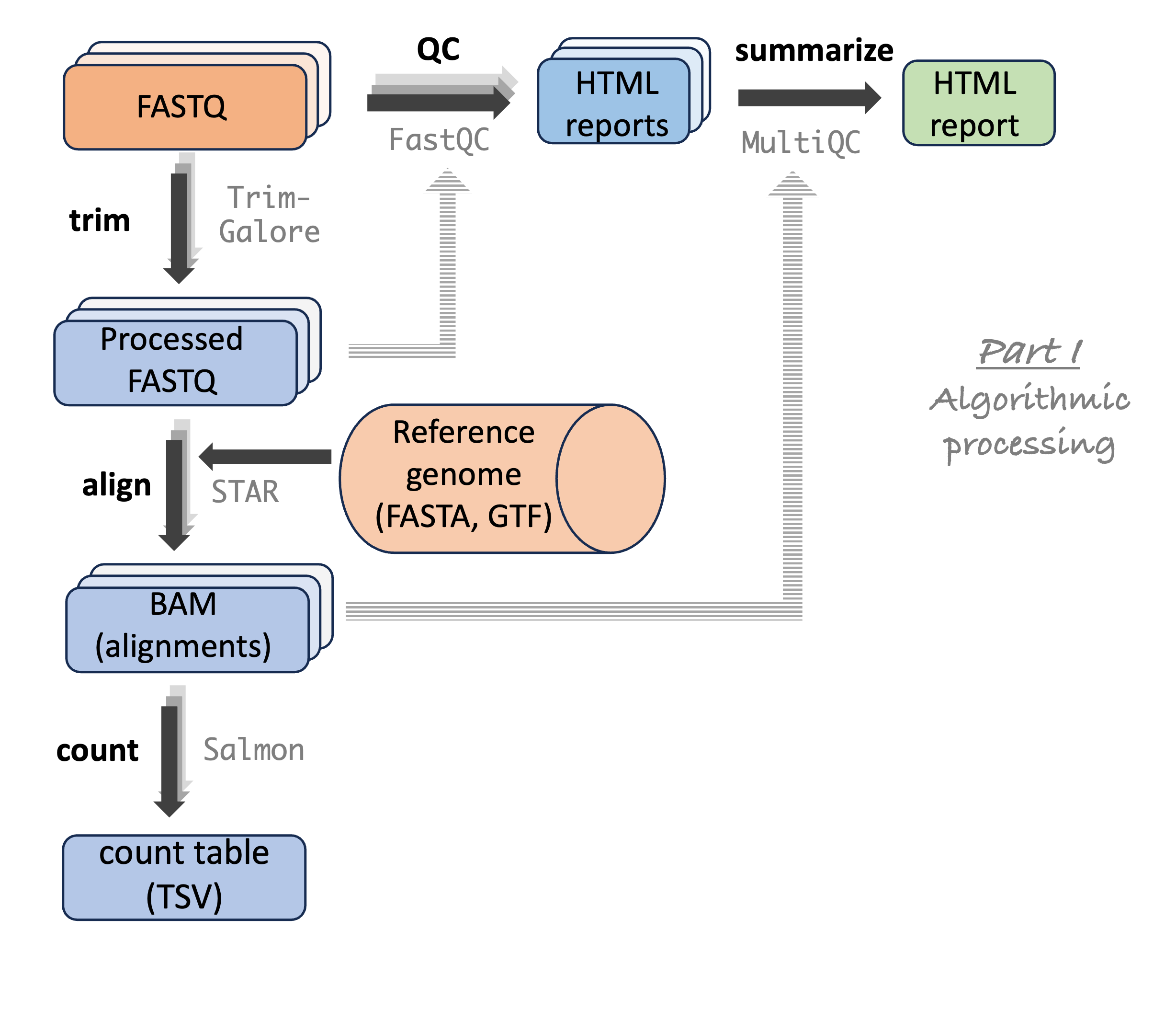
Analysis stage I: from reads to gene counts
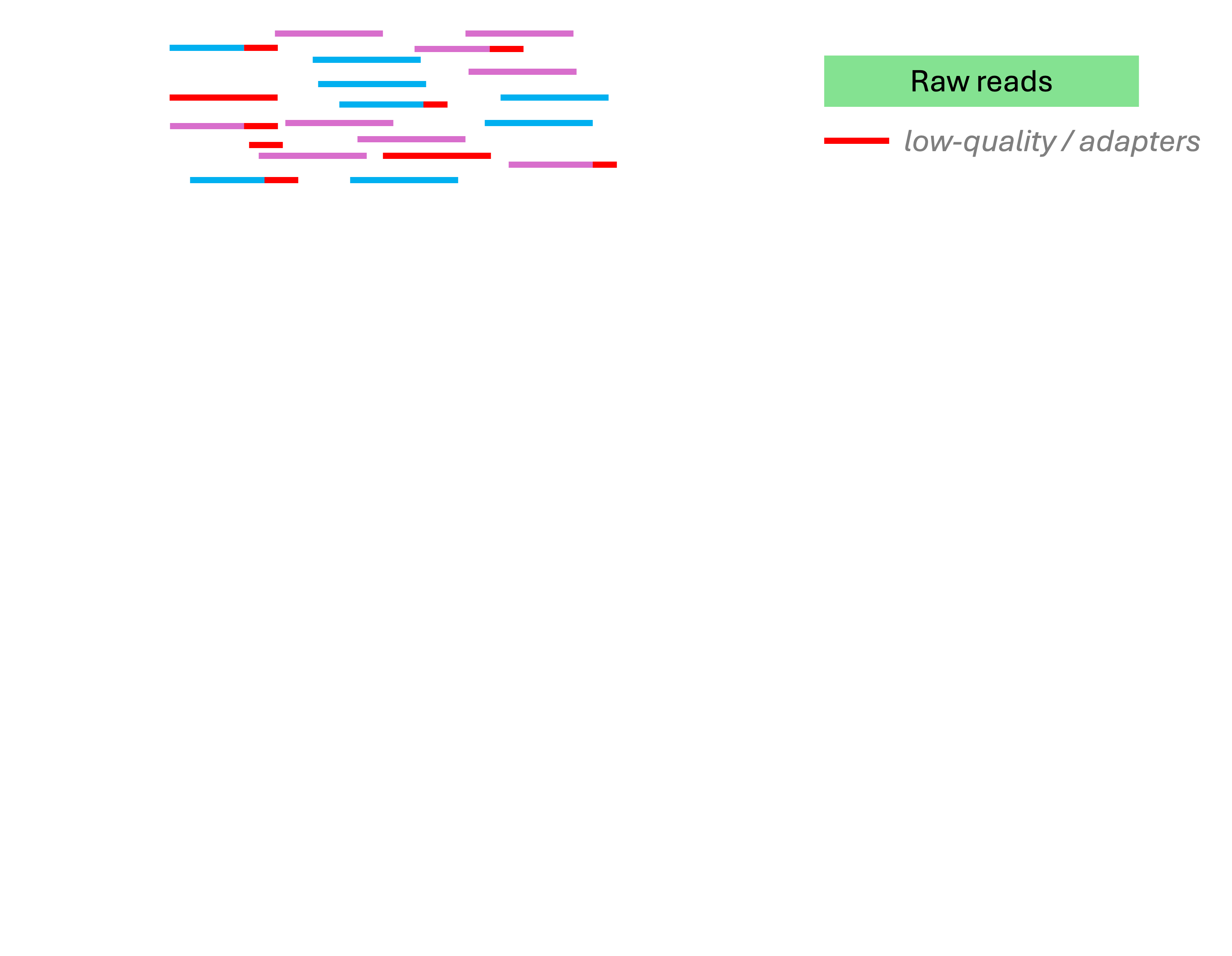
Analysis stage I: from reads to gene counts (cont.)
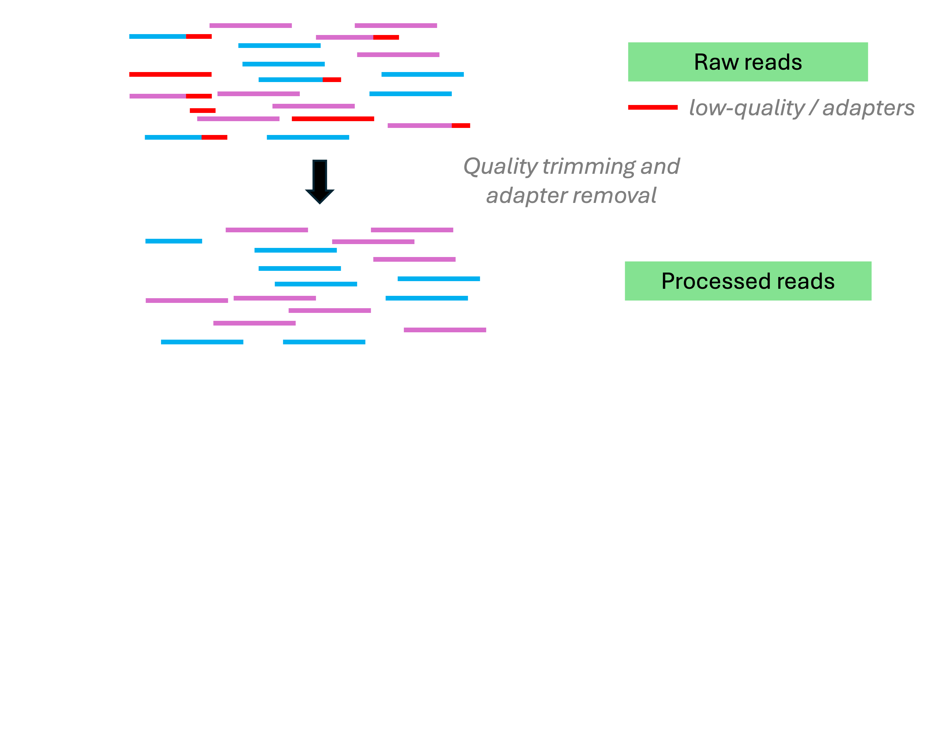
Analysis stage I: from reads to gene counts (cont.)
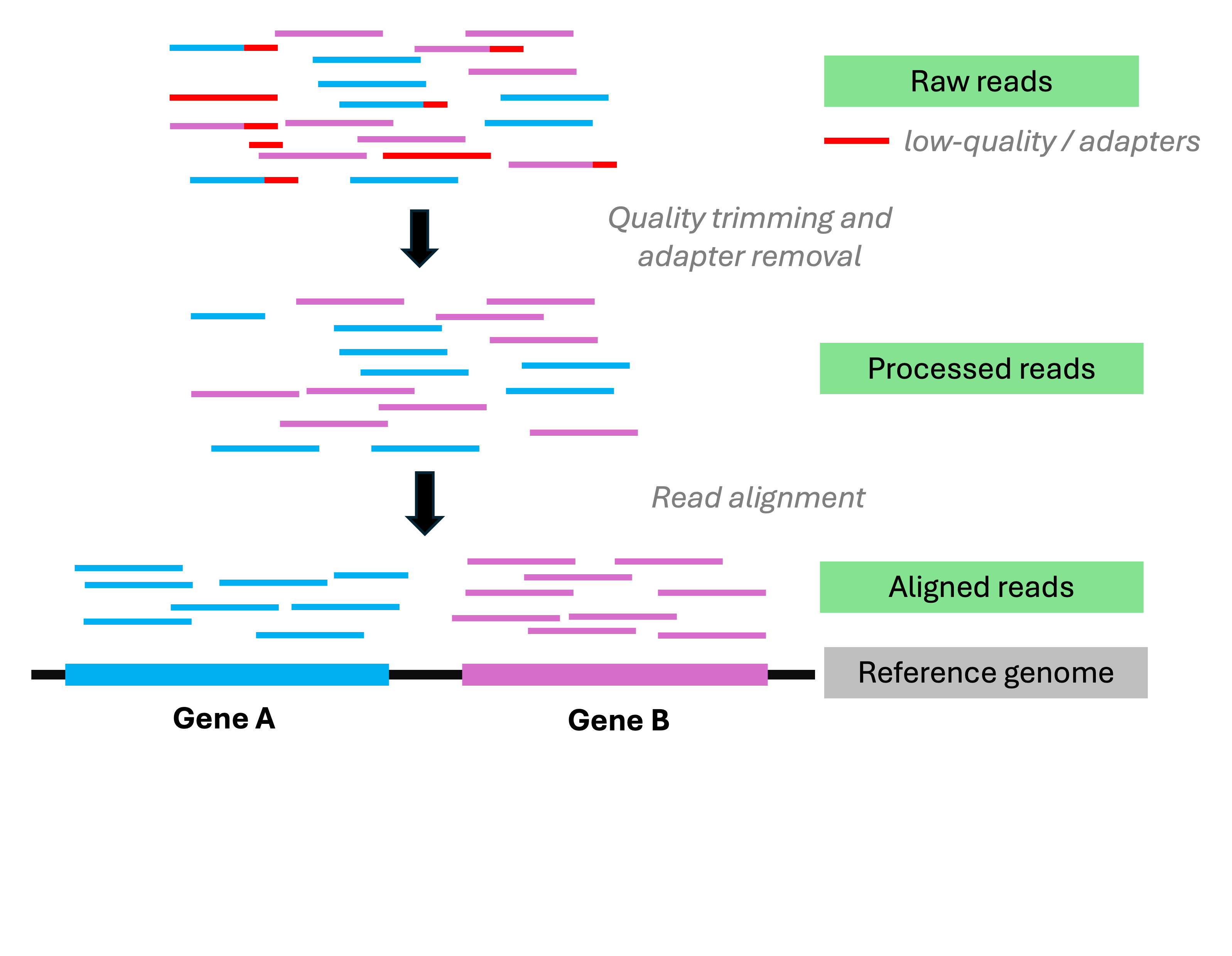
Analysis stage I: from reads to gene counts (cont.)
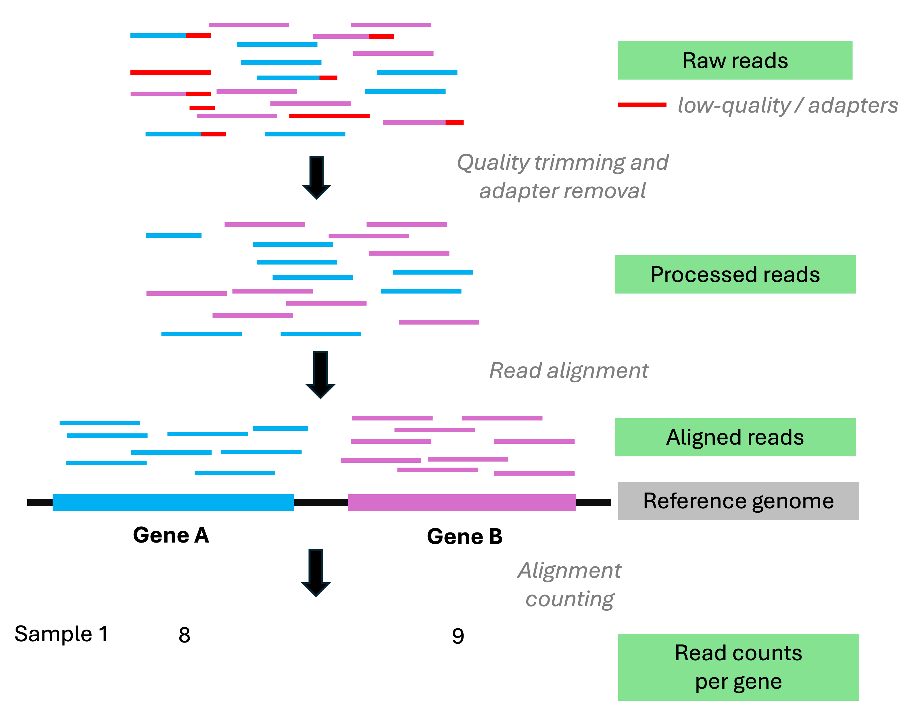
Analysis stage I: from reads to gene counts (cont.)
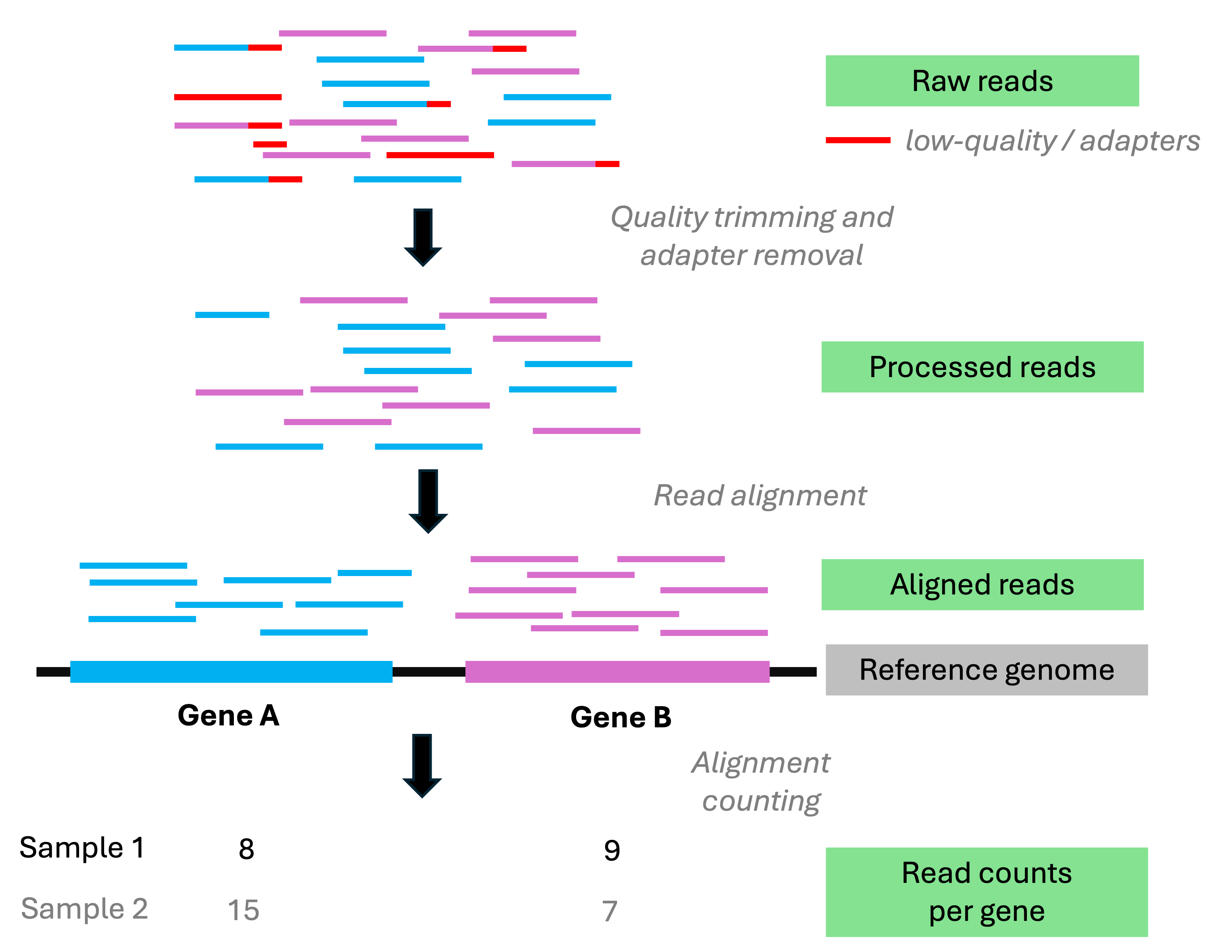
Analysis stage I: from reads to gene counts (cont.)
This is what the Adobe Firefly AI came up with when I tried to get it to help me with producing the diagram on the previous slide 👌 💯
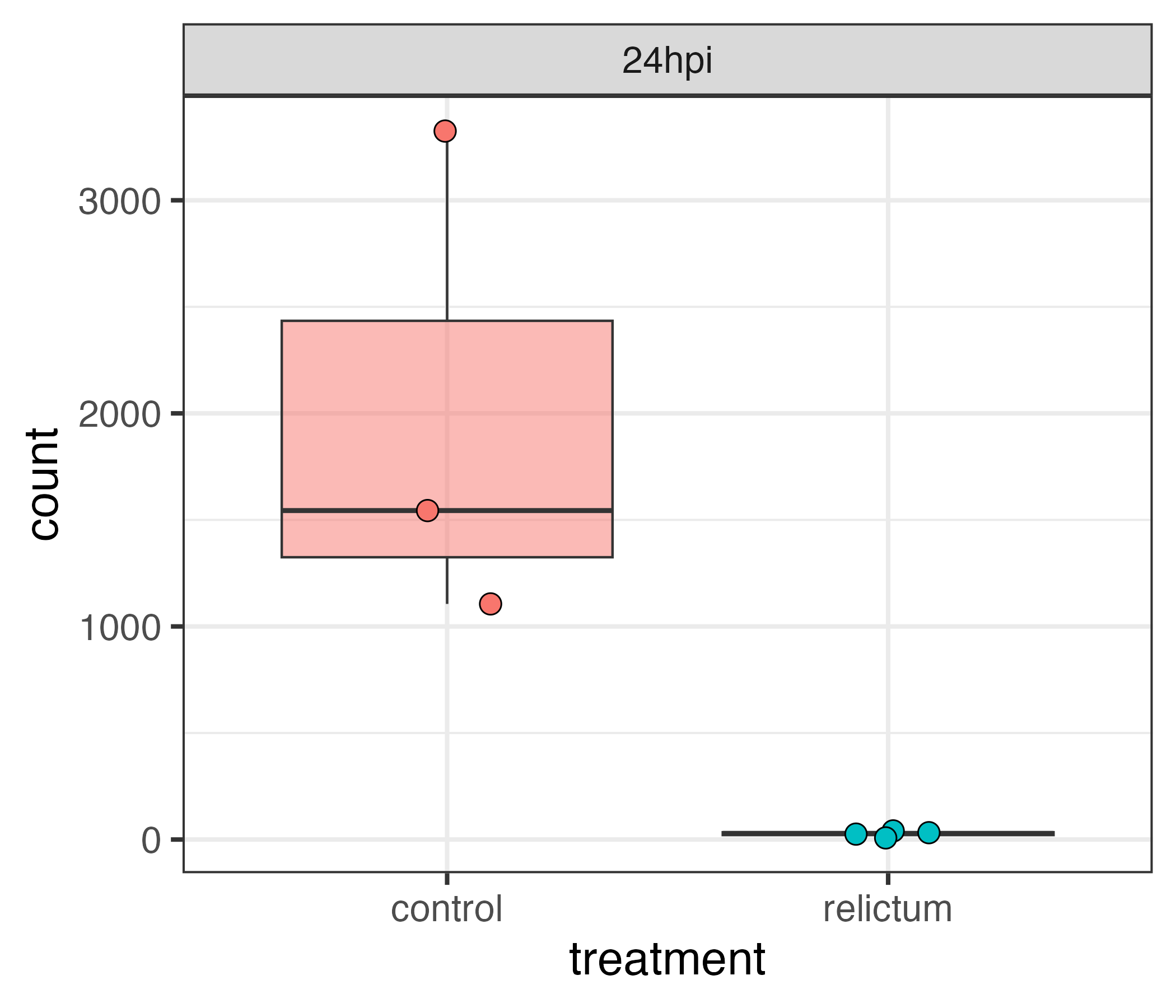
Analysis stage II: gene count analysis
A comparison of gene counts between treatments to see which genes differ in expression levels between treatments. For example, see the plot below for gene counts for a single gene:
Sequencing technology development timeline
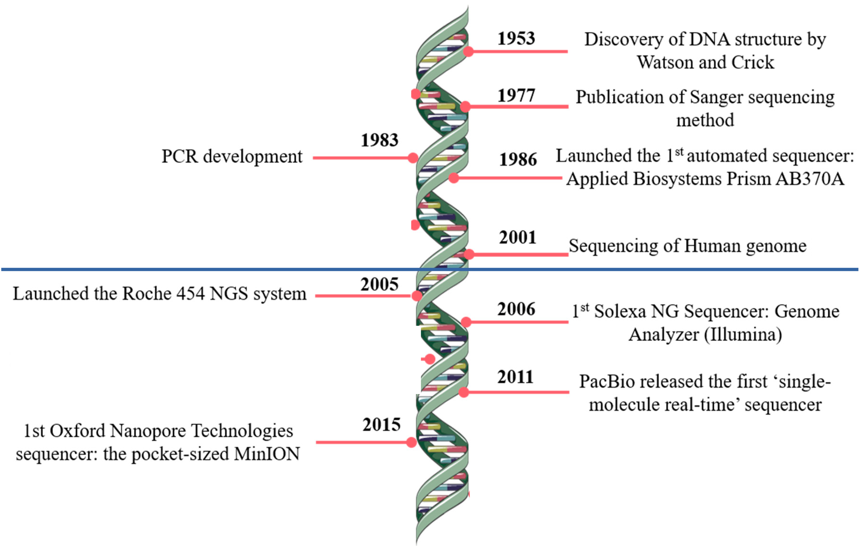
Modified after Pereira, Oliveira, and Sousa (2020)
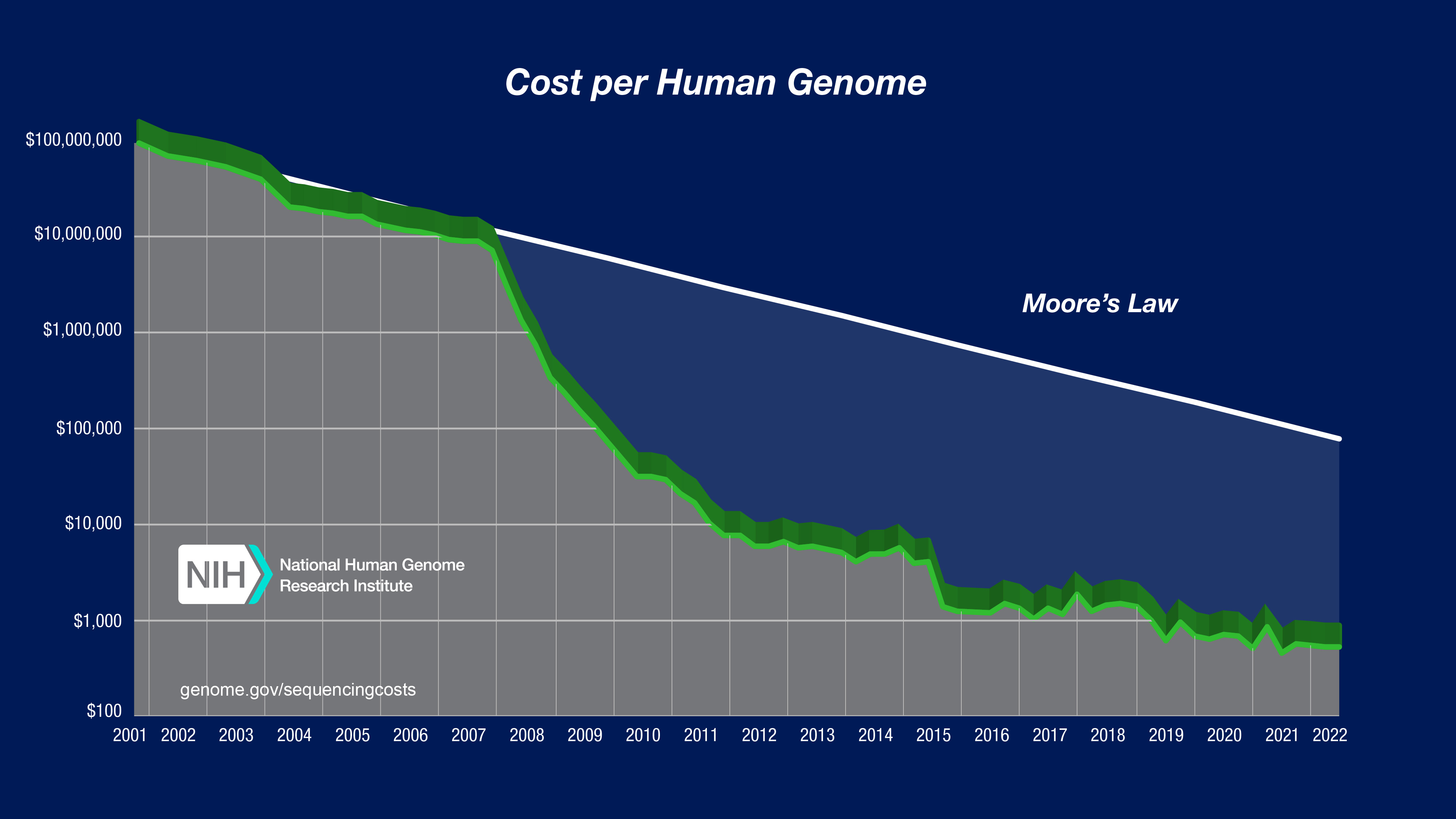
Sequencing costs have declined sharply
…with the advent of HTS.
HTS applications
From Lee (2023)
The sequencing process: Illumina
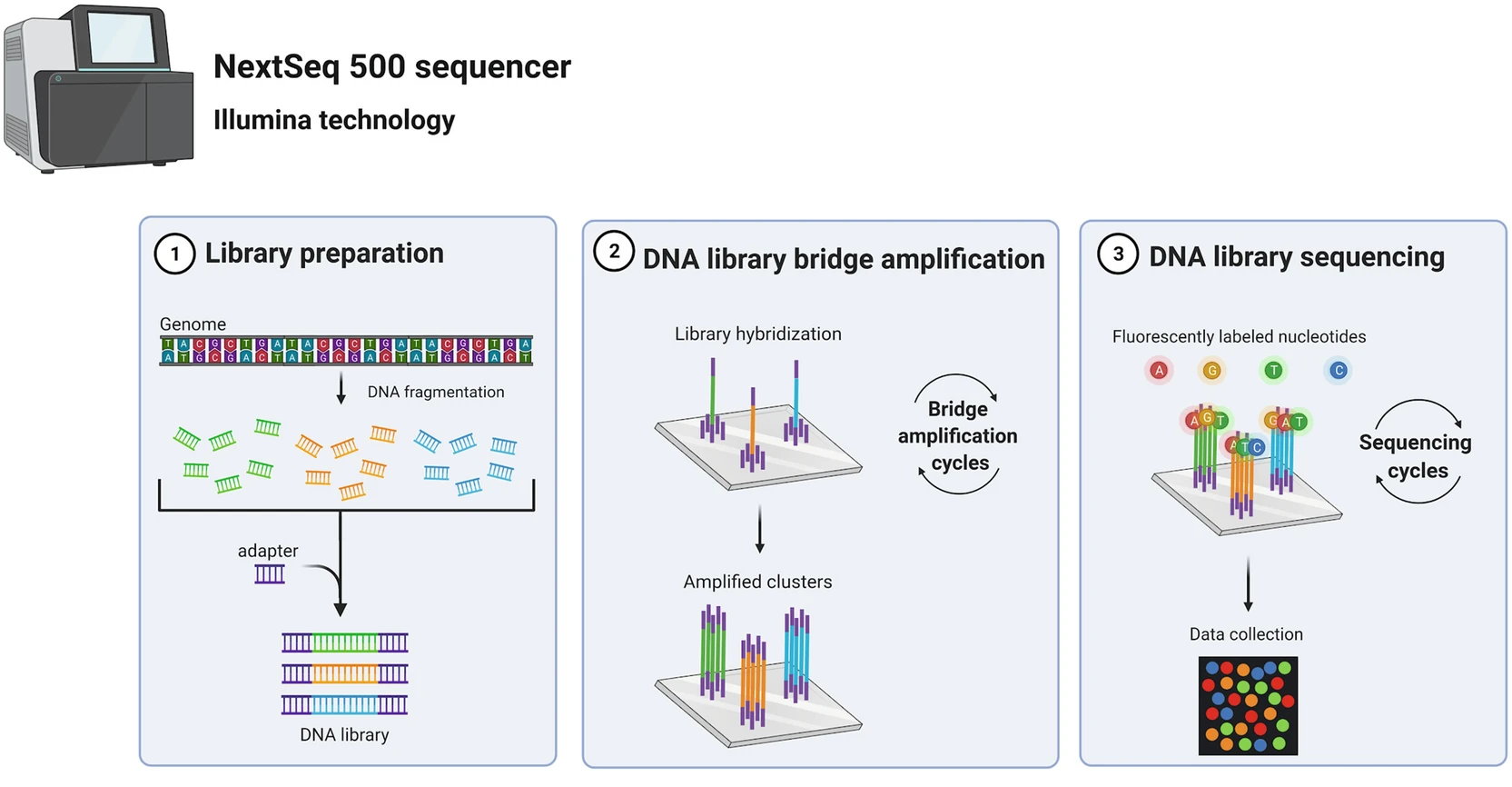
From Poinsignon et al. (2023)
The sequencing process: Oxford Nanopore
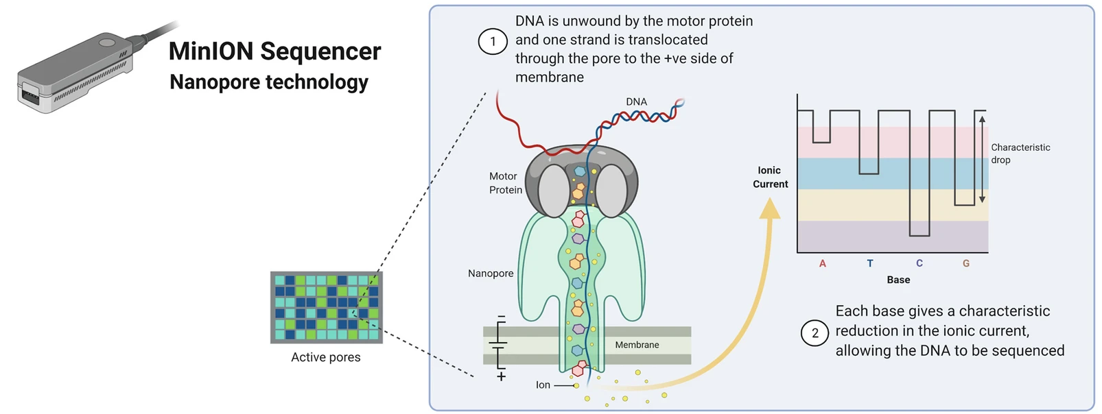
From Poinsignon et al. (2023)
Correcting sequencing errors
Inferring the sequence of the source DNA despite the presence of sequencing errors is attempted by sequencing every base multiple times, i.e. obtaining a so-called “depth of coverage” greater than 1:
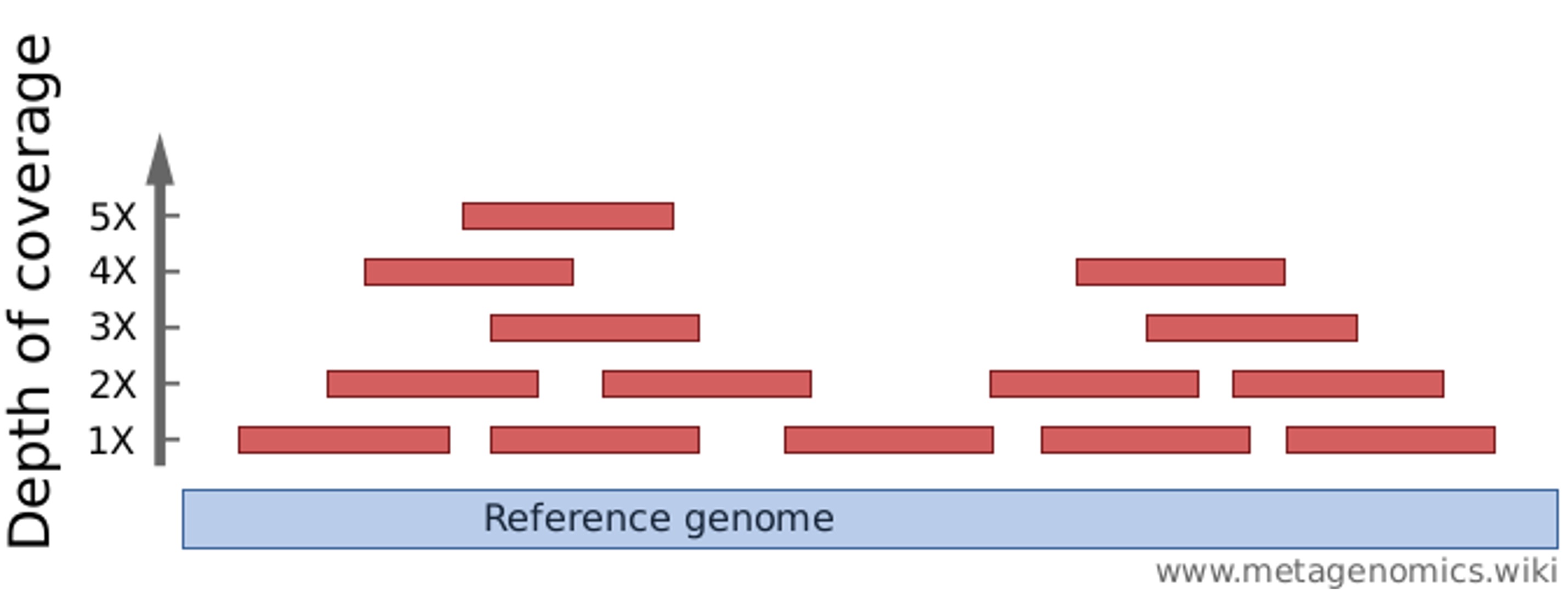
This process is complicated by genetic variation among and within individuals.
Typical depths of coverage: ~50-100x for genome assembly; 10-30x for resequencing.
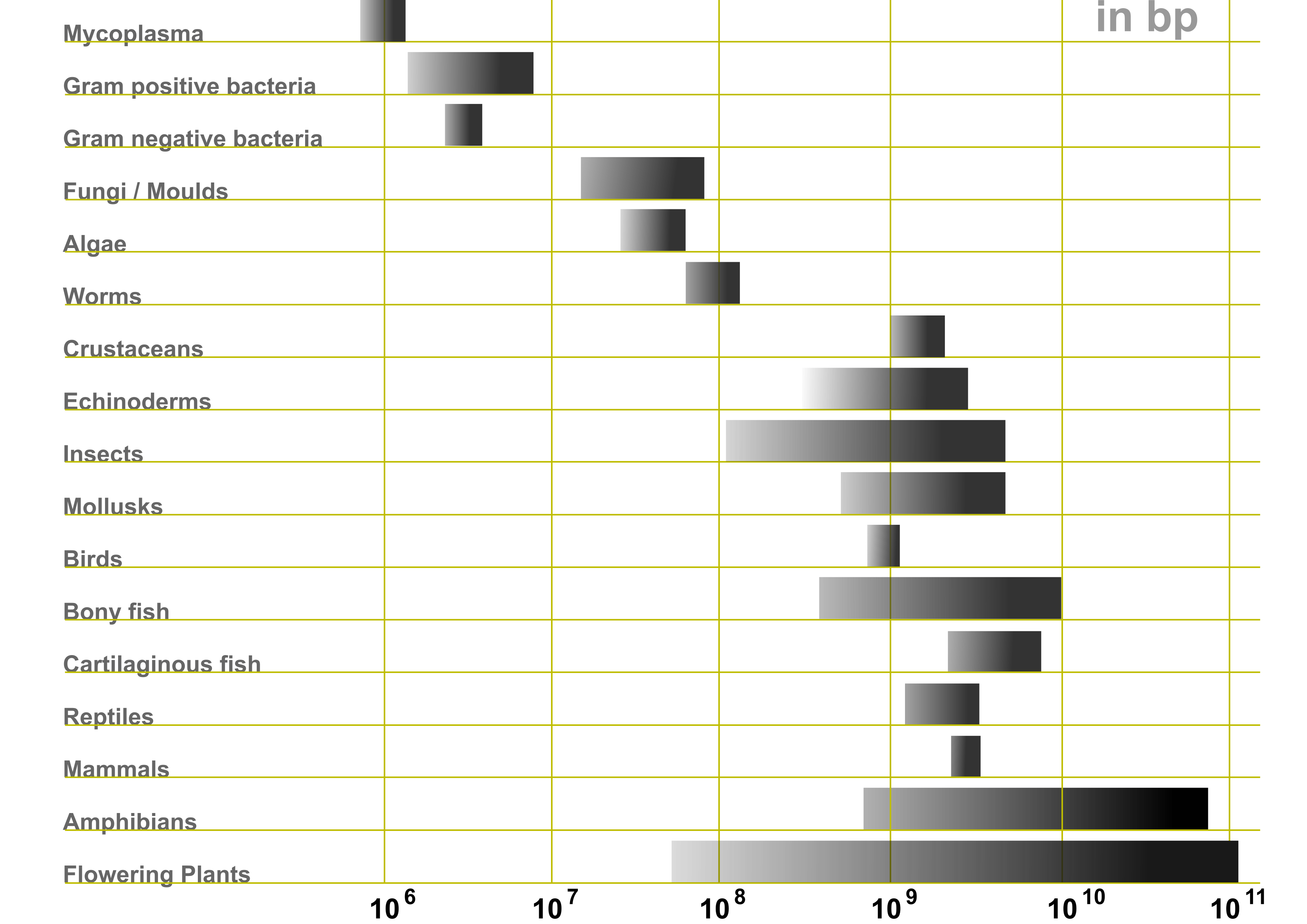
Genome size variation
Growth of genome databases
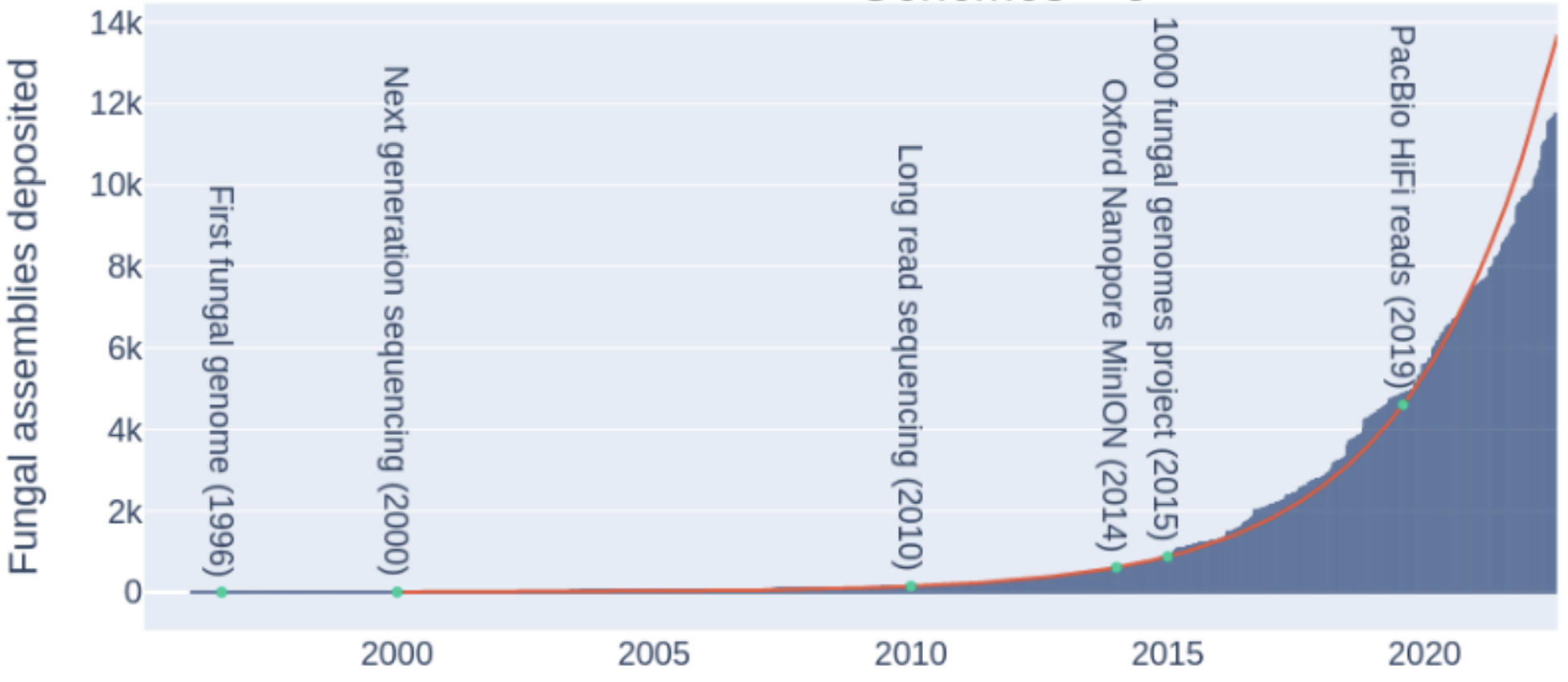
Konkel and Slot (2023)
From samples to reads for RNA-Seq
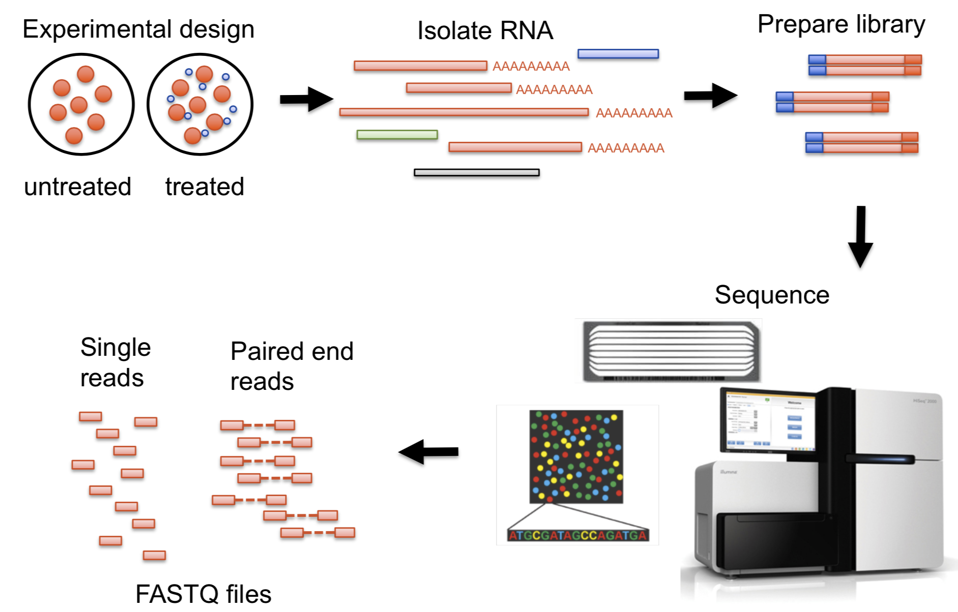
Overview of all key RNA-Seq analysis steps
Overview of all key RNA-Seq analysis steps (cont.)
Overview of all key RNA-Seq analysis steps (cont.)